In this paper, we present a topology optimization algorithm developed in Wolfram Mathematica, designed to generate structurally optimal objects capable of withstanding arbitrary forces under user-defined boundary conditions. By integrating custom penalty functions and a novel dual-objective formulation, our approach extends beyond traditional engineering frameworks, incorporating elements of computational aesthetics into the optimization process. This fusion allows us to explore how artistic principles - such as spatial harmony, dispersion, and visual balance - are effected by and influence material distribution and structural form. When extended into three dimensions, the algorithm reveals its practical potential: we analyze stress resistance and visualize force distribution to assess the real-world viability of these generated structures. Through this, we not only optimize for performance but also expand the boundaries of design itself.
Introduction
Introduction
Topology optimization represents a fundamental shift in structural design philosophy. Instead of beginning with a fixed geometry and manually adjusting its boundaries, we start with a full design domain - essentially a block of raw material - and allow mathematics to determine where material congregate and where it should be removed. This process of material redistribution, driven by physical constraints and performance goals, enables the creation of forms that are both efficient and often unexpectedly elegant. It has transformed industries such as aerospace, automotive, and civil engineering, leading to significant weight reductions while preserving or even enhancing structural integrity.
The specific method implemented in this project is based on the Solid Isotropic Material with Penalization (SIMP) framework. In SIMP, each finite element in the mesh is assigned a density variable ρ, ranging continuously from 0 (void) to 1 (solid). The core insight of SIMP lies in its penalization algorithm: intermediate densities are discouraged, effectively forcing the solution toward discrete, binary-like outcomes. This encourages clean designs composed of clear solid and void regions.
What makes this method especially powerful is its inherent flexibility. The continuous nature of the density field allows us to define custom penalty functions that go beyond traditional stress and compliance criteria. In this project, we leverage that flexibility to embed aesthetic constraints into the optimization process, encouraging material distributions that not only perform well mechanically but also exhibit visual coherence, dispersion, and formal balance. Through this fusion of structural logic and computational aesthetics, we explore a new paradigm where engineering performance and artistic intention can coexist in the same generative framework.
The specific method implemented in this project is based on the Solid Isotropic Material with Penalization (SIMP) framework. In SIMP, each finite element in the mesh is assigned a density variable ρ, ranging continuously from 0 (void) to 1 (solid). The core insight of SIMP lies in its penalization algorithm: intermediate densities are discouraged, effectively forcing the solution toward discrete, binary-like outcomes. This encourages clean designs composed of clear solid and void regions.
What makes this method especially powerful is its inherent flexibility. The continuous nature of the density field allows us to define custom penalty functions that go beyond traditional stress and compliance criteria. In this project, we leverage that flexibility to embed aesthetic constraints into the optimization process, encouraging material distributions that not only perform well mechanically but also exhibit visual coherence, dispersion, and formal balance. Through this fusion of structural logic and computational aesthetics, we explore a new paradigm where engineering performance and artistic intention can coexist in the same generative framework.
Global Simulation Parameters
Global Simulation Parameters
Controlling the behavior of the algorithm.
First, we define a set of base parameters. These values shape the material behavior, smoothing, and overall progression of the topology optimization.
Material Properties and Physical Parameters
Material Properties and Physical Parameters
Materials behave differently under load. When you stretch a rubber band, it gets thinner - this sideways shrinking is captured by Poisson’s ratio. Most metals have a Poisson’s ratio around 0.3, meaning they contract sideways by about 30% of how much they stretch lengthwise.
In continuum mechanics terms, Poisson’s ratio (ν) is defined as the negative ratio of transverse to axial strain: ν = -ε_transverse/ε_axial. This fundamental elastic constant completely characterizes the linear elastic behavior of the isotropic materials we will work with.
The volume fraction constraint represents our material budget, or the maximum percentage of the design domain that can be filled with material.
In continuum mechanics terms, Poisson’s ratio (ν) is defined as the negative ratio of transverse to axial strain: ν = -ε_transverse/ε_axial. This fundamental elastic constant completely characterizes the linear elastic behavior of the isotropic materials we will work with.
The volume fraction constraint represents our material budget, or the maximum percentage of the design domain that can be filled with material.
Defining Poisson’s Ratio.
In[]:=
poissonRatio = 0.3;
Allocating starting available material to the frame.
volumeFraction = 0.4;
Numerical Stability Parameters
Numerical Stability Parameters
Imagine trying to divide by a very small number - as it approaches zero, the result approaches infinity, causing mathematical problems. Similarly, when an element has near-zero density (almost void), it can cause mathematical instabilities.
Additionally, without proper filtering, the optimizer might create impractical checkerboard patterns (alternating solid-void elements). This occurs because checkerboard patterns artificially increase the structural stiffness, making them appear optimal to the algorithm even though they’re physically not optimal.
Additionally, without proper filtering, the optimizer might create impractical checkerboard patterns (alternating solid-void elements). This occurs because checkerboard patterns artificially increase the structural stiffness, making them appear optimal to the algorithm even though they’re physically not optimal.
The minimum density prevents complete void elements, maintaining numerical stability.
In[]:=
minimumDensity = 0.3;
The filter sigma controls spatial filtering to ensure smooth designs.
In[]:=
filterSigma = 0.8;
Optimization Control Parameters
Optimization Control Parameters
Topology optimization is inherently non-convex, which means that the path to the optimal solution matters. Aggressive updates can cause oscillations and sub-optimal outputs, while conservative updates converge slowly, resulting in long generation times. The algorithm uses a two-level iteration scheme: outer iterations for major design updates and inner iterations for smoothing and stabilization. Additionally, in order to create a smooth, generative design, maxMove is used as a control - ensuring that any given cell does not jump by a certain fraction of density at a time.
Specifies the maximum change in material density per iteration. The value is a fraction of density between 0 (void) and 1 (solid).
In[]:=
maxMove = 0.3;
Next, we define how many iterations our algorithm will go through. In this case, we set a minimum and a maximum iteration size, in order to counter under/overshooting the time needed to compute.
Specifying the range of evolutions the program is permitted to take.
In[]:=
minIters = 30;maxIters = 200;
Inner iterations allow for gradual adjustments to the material layout within each main step. This makes the updates smoother and more stable, especially when balancing multiple constraints like material usage and smoothness.
Sets how many smaller update steps/changes occur within each main design cycle. The value determines how gradually the material layout evolves.
In[]:=
innerIters = 100;
Iterative Parameters
Iterative Parameters
Topology optimization is an iterative process that needs clear stopping criteria. Without proper convergence checks, the algorithm might terminate prematurely (missing better solutions) or run indefinitely (wasting computational resources). These parameters implement a multi-criteria stopping strategy: the design must be sufficiently discrete (mostly 0s and 1s), stable over multiple iterations, and show minimal change. This ensures the solution has genuinely converged rather than temporarily stalled or is left unfinished.
In[]:=
convergenceThreshold = 0.95; binaryThreshold = 0.1;convergenceWindow = 5;densityChangeTolerance = 0.001;
Computational Aesthetics
Computational Aesthetics
The influence of aesthetics on engineering, and its implications in topological optimization.
The parameters for our optimization have clearly been set up. Now, it is a question of what we can do to take it a step further. After all, the intermediate between form and function is almost always more interesting and practical in the real world, so it is imperative that we show for it through application of “beauty” parameters. Not just optimized for function, but also for form.
These dispersion penalties shape how material distributes across the design space. Without them, optimization tends to create highly concentrated structures - mathematically optimal but often impractical. The dispersal penalty encourages material to spread out, creating more distributed load paths and redundancy. The nonlinearity parameter controls how aggressively the algorithm penalizes clustering - higher values create stronger pressure for distribution. The checkerboard penalty targets the alternating solid-void patterns that are artifacts rather than true optimal designs.
These dispersion penalties shape how material distributes across the design space. Without them, optimization tends to create highly concentrated structures - mathematically optimal but often impractical. The dispersal penalty encourages material to spread out, creating more distributed load paths and redundancy. The nonlinearity parameter controls how aggressively the algorithm penalizes clustering - higher values create stronger pressure for distribution. The checkerboard penalty targets the alternating solid-void patterns that are artifacts rather than true optimal designs.
The dispersal penalty weight adds a secondary objective encouraging material distribution. The neighborhood radius defines how locally the algorithm evaluates concentration. The nonlinearity makes the penalty much stronger for dense clusters. The checkerboard penalty suppresses alternating patterns.
In[]:=
dispersalPenaltyWeight = 0.2;dispersalNeighborhoodRadius = 2.0;dispersalNonlinearity = 3.0;checkerboardPenalty = 0.1;
Structured Playground Dimensions
Structured Playground Dimensions
Creating the sandbox for our code.
The image resolution size defines the base resolution of the design grid. A larger value creates a finer mesh, allowing for more geometric detail in the final structure. A smaller value results in a coarser design with fewer elements.
Sets the resolution scale used to determine the number of elements in the design grid. The value is a positive integer that is later multiplied by some given aspect ratio.
In[]:=
imgResolutionSize = 40;
The horizontal and vertical element counts are computed by multiplying the pair {4, 1} with the resolution multiplier. This multiplication is applied component-wise: the width becomes four times the resolution, and the height becomes one times the resolution. If the resolution is 40, the resulting grid has 160 elements in the horizontal direction and 40 in the vertical. The greater the resolution size, the greater the clarity and cost.
Scales the {4, 1} aspect ratio by the resolution multiplier. The result gives the total number of elements in the x (width) and y (height) directions.
{elemWidth, elemHeight} = {4, 1}*imgResolutionSize
Out[]=
{160,40}
Each quadrilateral element is defined by four corner nodes. Because nodes are shared between neighboring elements, the number of nodes will always be one more than the number of elements in each direction.
Adds 1 to both the width and height of the element grid to determine how many unique nodes are needed to define the corners of all elements.
{nodeWidth, nodeHeight} = {elemWidth, elemHeight} + 1
Out[]=
{161,41}
When working with structured grids, it’s helpful to convert a 2D layout (rows and columns) into a 1D list that preserves row-wise ordering. This allows for easier indexing and mapping of grid-based functions over arrays.
Defines a helper function that evaluates a function f[i,j] over a 2D grid of size dims, transposes it, and flattens it into a 1D list of outputs. The result is a list of values ordered from bottom-left to top-right across the grid.
Node and Element Indexing
Node and Element Indexing
Keeping track of the cells.
Each node in the grid can be uniquely identified by its position in the structured array of mesh points. These are typically stored as (i,j) index pairs for later use. This list serves as the index-able set of all points where displacements, forces, and boundary conditions will be applied.
Uses the flattenArray function to generate a full list of 2D node index pairs, ordered row-wise. Each pair represents the grid location of one node in {i, j} format.
nodes=N@flattenArray[{##}&,{nodeWidth,nodeHeight}];Short[nodes]
Out[]//Short=
{{1.,1.},{2.,1.},{3.,1.},{4.,1.},{5.,1.},{6.,1.},{7.,1.},6587,{155.,41.},{156.,41.},{157.,41.},{158.,41.},{159.,41.},{160.,41.},{161.,41.}}
Each quadrilateral element is defined by the indices of its four corner nodes, ordered consistently (e.g. counterclockwise). This list defines how local elements map to global node positions in the mesh.
For each element located at (i, j), calculates the indices of its four corner nodes based on grid position. The result below is a list of four node indices, each corresponding to one quadrilateral.
elems=flattenArray[With[{k=#1+#2*nodeWidth},{k-nodeWidth,k-elemWidth,k+1,k}]&,{elemWidth,elemHeight}];Short[elems]
Out[]//Short=
{{1,2,163,162},{2,3,164,163},{3,4,165,164},{4,5,166,165},{5,6,167,166},6391,{6436,6437,6598,6597},{6437,6438,6599,6598},{6438,6439,6600,6599},{6439,6440,6601,6600}}
Setting Up The Problem
Setting Up The Problem
The Problem that the Algorithm will respond to.
In structural analysis, boundary conditions define how and where the structure is anchored. This example selects the midpoint of both the left and right vertical edges as fixed points. By constraining these two nodes, the structure is prevented from drifting or rotating, while still allowing flexibility in its shape outside of these conditions. The idea behind these conditions are to simulate a real-life scenario, the support - valley - support in a bridge, with a downwards force simulating the weight of the bridge itself.

Setting up the boundary conditions as follows:
The middle row is found by dividing the total node height by two and rounding up. The left and right edge nodes in that row are then calculated by starting from the first and last node in a row (1, nodeWidth) and shifting up by the number of rows needed to reach the middle.
In[]:=
midRow = Ceiling[nodeHeight/2];midEdgeNodes = {1, nodeWidth} + (midRow - 1)*nodeWidth;
Collects the X and Y displacement indices for the midpoint support nodes and combines them into a single list of fixed degrees of freedom (AKA: the corresponding elements/nodes will never change)
In[]:=
fixedNodesDofs = Union[(2*midEdgeNodes) - 1, 2*midEdgeNodes];
Setting up the point force(s) as follows:
The node receiving the force is calculated by first finding the center of the bottom row, then shifting up one full row by adding nodeWidth. The load is assigned as a vector {0(x), -1(y)} meaning it acts purely in the negative Y-direction (downward), with unit magnitude. The load is wrapped in a list to fit the program’s expected input format for point forces: [Node, Force direction]
bottomSecondRowNode = Ceiling[nodeWidth/2] + nodeWidth;pointLoads = {{bottomSecondRowNode, {0, -1}}}
Out[]=
{{242,{0,-1}}}
While this is a good simple way to add a point force, it is still not completely accurate. With a real bridge, the force of the weight is not simply just at the center of the bridge, but rather the force increases as it gets closer to the center. In order to model this, we implement a binomial function that we can scale to fit a unit force.
Out[]=
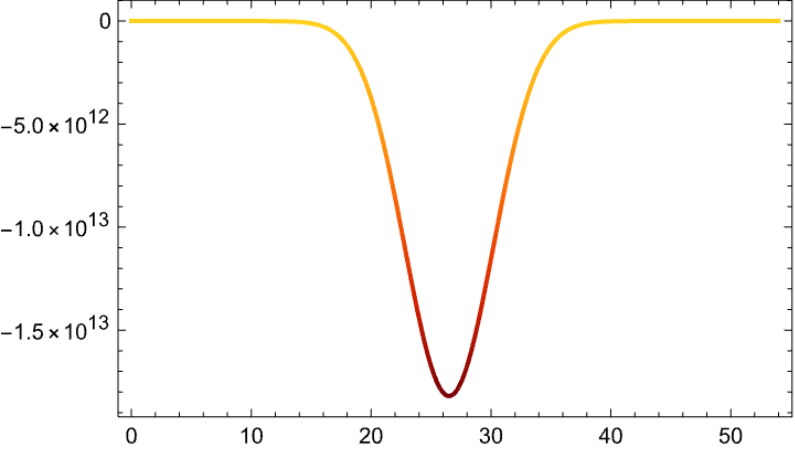
The code for the distributed force is as follows.
Distributed Force
Once the mesh is created, the forces are in place, and the selected nodes are fixed, we look for bookkeeping variables to track the problem size. The volume constraint is enforced by limiting how many elements can be solid. With a 40% volume fraction, only 2,560 of our 6,400 elements can be solid material - the remaining 3,840 must be set to minimum density.
We proceed with calculating the total number of elements and nodes in the mesh after mesh generation.
Calculates how many elements must be set to minimum density to satisfy the volume constraint. We will check with this value later in the algorithm.
Algorithmic Anomaly Avoidance (AAA)
Algorithmic Anomaly Avoidance (AAA)
Refining the Outcome.
In this optimization, sensitivities represent how the objective function changes with respect to each element’s density - essentially the gradient ∂c/∂ρ. Raw sensitivities often suffer from numerical problems that manifest themselves as pixelated/checkerboard patterns. The filter applies spatial smoothing using Gaussian filtering, ensuring neighboring elements have similar sensitivities. This creates a length scale in the design and prevents features smaller than the filter radius - essentially improving the “relationship” between elements. This filtering has an anisotropic nature (larger smoothing horizontally than vertically), which helps preserve vertical load paths while also smoothing horizontal variations.
Reshapes the 1D sensitivity array into a 2D grid, applies Gaussian filtering with different strengths in each direction, then flattens back to 1D. The “Reversed” padding mirrors values at boundaries.
The routine first shapes the one-dimensional list of element densities into a 2-D grid that mirrors the physical layout of the FEM; this lets every element respect neighbourhood relationships rather than treating other elements as an unrelated list. A Gaussian blur is then applied to that grid, giving each element a smooth local-average density - think of it as asking “how solid is the material around me?” but calculated with a mathematically well-behaved filter that avoids sharp cut-offs. The element’s own density and that neighbourhood average are each raised to a user-chosen power (dispersalNonlinearity), then multiplied; this exaggerates situations where both the element and its surroundings are simultaneously dense, producing the classic concentration measure that drives material away from clumps.
Computes local density averages using Gaussian filtering, raises both local and average densities to the nonlinearity power, scales by normalized element energies, and returns the penalty term.
This next conversion helper waits until a minimum number of outer iterations have passed, and then applies two independent tests. First it measures how “binary” the design is: counting what fraction of elements now lie very close to 0 or 1 (below threshold or above threshold). Next, it looks at stability, recording the maximum change since the previous iteration, and computes the average of those maxima over recent steps. If the structure is mostly binary and its density field has stopped moving , or if all changes have fallen an order of magnitude below that tolerance, the function returns True, signalling convergence; otherwise it returns False so the optimization continues. Taken together, these criteria make sure the algorithm only stops when the topology has settled into a crisp, clear pattern with further iterations yielding negligible changes to the design.
In finite element analysis, we need to understand how each element responds to forces. The element stiffness matrix is like a spring constant for a 2D element - it tells us how much the element’s nodes will move when a given force is applied. For our quadrilateral (4-sided) elements, each corner node can move in two directions (x and y), giving us 2 degrees of freedom (DOFs) per node. With 4 nodes total, we have 8 DOFs per element, resulting in an 8×8 stiffness matrix. This matrix encodes how a force on any node affects the displacement of all nodes.
Due to the physics of elastic deformation, the matrix is always symmetric: the force at node i due to displacement of node j equals the force at node j due to displacement of node i.
Rather than computing complex integrals of shape functions, we use a pre-integrated analytical solution for a unit square element. This gives us just 8 unique values that, through symmetry, fill the entire 64-entry matrix.
Due to the physics of elastic deformation, the matrix is always symmetric: the force at node i due to displacement of node j equals the force at node j due to displacement of node i.
Rather than computing complex integrals of shape functions, we use a pre-integrated analytical solution for a unit square element. This gives us just 8 unique values that, through symmetry, fill the entire 64-entry matrix.
Computes the 8 unique stiffness values in a 8x8 matrix, creates an index pattern for the symmetric matrix structure, and maps values to their positions.
The heart of finite element analysis lies in solving the fundamental equation KU = F - the global stiffness matrix times displacements equals applied forces. In topology optimization, we’re interested in how much elastic energy each element stores under load, as this drives the optimization process. Elements under high stress should attract material, while unstressed regions can afford to lose it. The SIMP method scales each element’s contribution by its density raised to a power, making intermediate densities inefficient and pushing the design toward solid-void solutions. This is the basis of the entire program: an element has high energy? Add material. An element has low energy, void it.
This function assembles the global stiffness matrix from element contributions, applies boundary conditions, solves for nodal displacements, and computes the strain energy in each element.
Building the global system from individual elements requires careful bookkeeping. Each element contributes to the global stiffness matrix at positions corresponding to its nodes’ degrees of freedom. Because most entries remain zero (each node only connects to its neighbors), we use sparse matrix storage. A sparse array allows for the code to only account for the filled numbers, disregarding the 0’s - taking up less space and increasing computational speed. The assembly process must also handle boundary conditions - fixed supports that constrain certain degrees of freedom. This step creates all the data structures needed for efficient repeated solving during optimization iterations.
Packaging all the values for the solver beforehand.
Topology optimization faces a fundamental challenge: we need to optimize densities constrained to [0,1], but constrained optimization is difficult. Often, we get density values over that range due to the code, but there is an easy fix. The solution is to transform to unconstrained design variables that can take any value from -∞ to +∞, to a hyperbolic tangent transformation: ρ = (1 + tanh(x))/2, essentially mapping unconstrained variables “x” to densities [0,1]. This ensures that we are able to simplify the values, while still keeping them relative to each other.
Implementing the code, and checking material usage through the volumeConstraintFunction to ensure no over/undershooting of material.
Even if the code does overshoot the deletion of low-energy cells, this code will be able to bring it back to the desired goal.
The Optimization Loop
The Optimization Loop
Where the simulation finally comes into fruition.
The optimization loop is where the magic happens. It iteratively adjusts element densities to minimize compliance (maximize stiffness) while satisfying the volume constraint. The algorithm uses a nested structure: outer iterations for major design updates and inner iterations for smoothing. This approach, combined with sensitivity filtering and adaptive step sizes, ensures convergence to a high-quality optimization to whatever constraints are given.
Note: Everything in this loop should be part of one cell, but for clarity, we will split it up to explain each portion.
Sets up the block with our parameters and bookkeeping variables.
Calculating the strain energy for each element, and multiplying buy the current density of the cell in order to get sensitivity, then applying the dispersion filter and calculating.
Inner Optimization Steps
Inner Optimization Steps
At the very start of the run, this block picks a cut-off energy that marks the boundary between elements that should be moved, and deleted. Then, it turns that cut-off into tiny step sizes that limit how much each element’s material density is allowed to change in the upcoming inner updates. In practice, this means every element - every square of the FEM - will move only a fraction away from its current density during the first cycle, controlling the smoothing and allowing the program to take it’s time when preforming inner optimization steps.
Defining lagrangeStepSize and adaptiveStepSize
This graph gives great insight into the cleverness of the lagrange multiplier; it presses the overall grid to change abruptly when farther away from the ideal “black and white” defined object, and slowly decreases it’s effect as the simulation gets closer and closer to the desired result. By the time the object has successfully converged, the lagrange multiplier is only a subtle constant that keeps the structure stable.
Note: this code is run later in the program: as the loop has to finish before it can be evaluated.
Now, we can move onto the inner loop.
Enter the inner looping algorithm.
Define the variables that will be updated and referenced throughout the inner loop.
Calculating update weights and new design variables. Affects the sensitivity of each element based on it’s design variables, pushing different elements differently to optimization: variables that are in the “uncertain”, or in the middle of density, will be assigned a higher density so that they may “choose” their side.
Implement weighted step-size.
Next, we move onto the volume constraint function preforming a variety of checks on the current volume of the overall design. Based on if the design is over or under the goal margin, we decrease or increase the lagrange multiplier, and if we reach the volume within a 0.1% margin, we break the loop early.
Implement constraint loop/checker.
Each inner iteration takes the volume-constrained design, gauges its total movement from the outer-loop start and breaks the loop if it breaches the volume cap, computes a derivative from the filtered densities, notes the expected advance from the current step size, and makes an attempt to converge the material safely with the reaction in comparison to the expected advance.
Implementing the step-size checker.
Converting back to density from design variables.
The graphs below represent the success of the optimization loop, showcasing the decreasing volatility after around 50 iterations and the adaptive nature of the algorithm itself.
Compliance Plot:
Density Error Plot:
Visualization Algorithm
Visualization Algorithm
Now, we can create the current iteration’s visualization. It first adds a raster image where the density grid is displayed - white represents void (density 0) and black represents solid material (density 1). If any elements have just become void in this iteration, it adds a red overlay layer. The MapIndexed function goes through the red flash grid and creates a red rectangle for each element that has a non-zero opacity value. The rectangle coordinates are calculated from the grid indices, with -1 adjustments because Mathematica’s graphics coordinates start at 0 while the array indices start at 1. The complete graphics object is then added to the animation frames list with a fixed size of pixels (based on the frame size) to ensure consistent playback.
Starting the visualization block
Logging metrics for graphing use
Before returning our optimization, we need to check if the code should either break or continue to update. We do this by updating the previous density with the current density, and then checking for convergence (if it is converged, there is no reason to continue the program)
Convergence Check
Finally, we can return the final output as well as our final frame, the optimized structure.
Returning the animation, the last frame of the animation, and if the structure has converged or not.
Analysing the Results
Analysing the Results
Now, let us observe our results. Remember, the red showcases elements being “removed”, white signifies an already removed element, and the gradient from grey to black showcases low and high stiffness, respectively.
Selecting a few “key” frames from the structure
The emergent structure of these formations are particularly interesting. Perfectly symmetrical, beautiful objects that don’t cluster, don’t randomize, and behave.
We can observe the fluidity of this algorithm by changing the volumeConstraint while keeping the rest of the parameters constant.
We can observe the fluidity of this algorithm by changing the volumeConstraint while keeping the rest of the parameters constant.
By running a ParallelTable of varying allotted material, we are able to iterate through volumeConstraints in order to showcase all the final results, storing them to a list.
We are able to create an animation from these final frames
As the density increases, one might expect the overall “beams” of the structure to simply increase in length. However, our dispersive filters counter this inherent behavior: driving the structure away from just simple, blocky shapes. This creates the phenomenon of “pocketing”, or the insertion of triangles throughout the structure, forming unique truss’s all over the design. Maintaining structural integrity while compensating for aesthetic appeal as well: this is a huge success. yoda67
Let us take a couple of frames to analyze.
By applying a color function to the array-plot, we are able to accurately visualize the energy levels throughout the structure as it evolves.
Temperature Map Visualization
We get a list back with the density visualized as colors, of which we can animate.
Interestingly enough, adjusting the dispersion filter enough gives us a completely different outcome in terms of design:
And finally, we are able to visualize how the structure of the optimization changes as the point load moves across a surface.
The Third Dimension
The Third Dimension
A 3-Dimensional Analysis
By taking a final frame of a given design, we are able to bring it up a dimension in order to analyse exactly how it preforms under a real force.
First, we define our variables in the 3rd dimension, and designate the material of titanium to our design, which is exactly the range of the Possion ratio we initially used.
The image of choosing, after applying a gaussian blur and adjusting the contrast to sharpen, and converting to a binary image (0’s and 1’s/only white and black)
We can create a function that transforms any given binary image into a extruded region.
This function will return us a region, but in order to preform the calculations we need, we must convert it to a boundary mesh region.
Defining the boundryMeshRegion.
Looking at the dimensions of the object.
We notice that this meshRegion is very large, as it is scaled by the amount pixels correlating to meters. To scale it down, we use region resize.
Resizing the truss to a manageable length and width - by a factor of 5.
Before we start the physical evaluations on the object, we must define a couple of parameters.
In order to have good points of force and boundary conditions, we must apply the forces/conditions to a region: not just a point. The mesh is not perfect, so this will accurately simulate a force over an area rather than a pixel.
Setting the “some” values which will be used to calculate crucial regions.
Using NDSolveValue to solve for the displacement.
Calculating for the strains and vonMisesStress.
We can visualize the vonMisesStress both on the outside and the inside of the structure.
The strains and equivalent strains can also be plotted.
Conclusion
Conclusion
In this project, we analyzed the field of topology optimization and explored its overlooked connections with art and aesthetics. We developed a novel optimization algorithm capable of integrating parameters from both engineering and visual design by utilizing the Solid Isotropic Material with Penalization (SIMP) technique. Through a series of simulations and visual evaluations, we confirmed the viability of our approach - not only in producing structurally sound forms under arbitrary loading and boundary conditions, but also in generating designs that exhibit visual coherence, spatial balance, and aesthetic intent.
Future Direction
Future Direction
Building on the foundation of this project, promising directions remain for future exploration. First, physical creation of the generated designs using a CNC machine would allow us to test structural performance and visual impact in tangible form - bridging the gap between digital theory and physical fabrication. Second, the algorithm could be extended to not just respond to force placement, but to actively optimize it for aesthetic outcomes, generating forms that are not only structurally sound but visually striking. Third, we aim to introduce explicit artistic constants - such as the golden ratio, rule of thirds, and symmetry heuristics - into the optimization process as tunable parameters, enabling a more direct and formal integration of design principles. Finally, the algorithm could be expanded into three dimensions, replacing square elements with volumetric cubes. This would vastly increase the complexity - and potential - of the structures, opening the door to spatial forms that exhibit both mechanical and sculptural beauty.
Acknowledgements
Acknowledgements
First, and most importantly, this project would not have been possible without the guidance and support of my mentor, Shenghui Yang, whose intelligence, dedication, humor, and deep love for science shaped not only my project, but also my passion for the work and the program itself. I could not have asked for a better mentor, and I am eternally grateful I had the opportunity to work with such a brilliant mind.
I would like to thank my advisors, Ethan Kong, Austin Jiang, and Gregory Roudenko for their immense help with the code and math behind this project, Ritvik Gupta for introducing me to this wonderful program in the first place, as well as the rest of the TAs in the program for their insight, encouragement, and commitment in making this program worthwhile. Their expertise and heartfelt trust in this vision pushed me forward and helped shape the project into what it ultimately became.
I would like to thank my advisors, Ethan Kong, Austin Jiang, and Gregory Roudenko for their immense help with the code and math behind this project, Ritvik Gupta for introducing me to this wonderful program in the first place, as well as the rest of the TAs in the program for their insight, encouragement, and commitment in making this program worthwhile. Their expertise and heartfelt trust in this vision pushed me forward and helped shape the project into what it ultimately became.
Citations
Citations
◼
Hu, Yifan. “Stress Propagation in a Truss Bridge.” Wolfram Demonstrations Project, Wolfram Research, 28 Sept. 2007, demonstrations.wolfram.com/StressPropagationInATrussBridge/.
◼
Krotkikh, Andrey. “Implementation of Topology Optimization Algorithms in Wolfram Mathematica.” Wolfram Community, Wolfram Research, 2016, community.wolfram.com/groups/-/m/t/1566977.
◼
“Understanding the Finite Element Method.” The Efficient Engineer, efficientengineer.com/finite-element-method/.
◼
O’Shaughnessy, Connor, Enrico Masoero, and P. D. Gosling. “Topology Optimization Using the Discrete Element Method. Part 1: Methodology, Validation, and Geometric Nonlinearity.” Meccanica, vol. 57, no. 6, 2022, pp. 1213–31. Springer, doi:10.1007/s11012-022-01493-w.
◼
Kong, Ethan. “[WSRP24] Optimization of the Thrust to Power Consumption Ratio of Ion Thrusters through Simulations.” Wolfram Community, Wolfram Research, 2023, community.wolfram.com/groups/-/m/t/3217524.
◼
Laarman, Joris. “Arm Chair.” Joris Laarman Studio, 2007, jorislaarman.com/work/arm-chair/.
◼
Gupta, Ritvik. “[WSRP24] Simulating the Flocking Behavior of Boids within a Parametrically Defined Vector Field.” Wolfram Community, Wolfram Research, 2023, community.wolfram.com/groups/-/m/t/3211600.
CITE THIS NOTEBOOK
CITE THIS NOTEBOOK
Intersections of form & function: The aesthetic dimension of topological optimization
by Yuvraj Chaudhary
Wolfram Community, STAFF PICKS, July 11, 2025
https://community.wolfram.com/groups/-/m/t/3503336
by Yuvraj Chaudhary
Wolfram Community, STAFF PICKS, July 11, 2025
https://community.wolfram.com/groups/-/m/t/3503336