CITE THIS NOTEBOOK: Inference of signaling mechanism from cellular responses to multiple cues by Soutick Saha, Wolfram Community, SEP 29 2022.
ORIGINAL ARTICLE: Saha, S., Moon, Hr., Han, B. et al. Deduction of signaling mechanisms from cellular responses to multiple cues. npj Syst Biol Appl 8, 48 (2022). https://doi.org/10.1038/s41540-022-00262-5.
ORIGINAL ARTICLE: Saha, S., Moon, Hr., Han, B. et al. Deduction of signaling mechanisms from cellular responses to multiple cues. npj Syst Biol Appl 8, 48 (2022). https://doi.org/10.1038/s41540-022-00262-5.
Original Article Abstract: Cell signaling networks are complex and often incompletely characterized, making it difficult to obtain a comprehensive picture of the mechanisms they encode. Mathematical modeling of these networks provides important clues, but the models themselves are often complex, and it is not always clear how to extract falsifiable predictions. Here we take an inverse approach, using experimental data at the cell level to infer the minimal signaling network. We focus on cells’ response to multiple cues, specifically on the surprising case in which the response is antagonistic: the response to multiple cues is weaker than the response to the individual cues. We systematically build candidate signaling networks one node at a time, using the ubiquitous ingredients of (i) up- or down-regulation, (ii) molecular conversion, or (iii) reversible binding. In each case, our method reveals a minimal, interpretable signaling mechanism that explains the antagonistic response. Our work provides a systematic way to infer molecular mechanisms from cell-level data.
Introduction
Introduction
Cell signaling is an intricate phenomena that occurs in response to a complex microenvironment involving multiple signals at the same time. The biochemical networks involved in the process can be incredibly complex and often incompletely characterized. Nonetheless, it is very important to understand the molecular mechanisms underlying complex cell behavior. To address this question we take the reverse approach in our paper. Starting with the surprising phenomena of antagonism, we systematically deduce the minimal and sufficient network(s) that can explain antagonism in cell behavior in response to two signals or inputs. Antagonism occurs when the response of the cell to individual inputs is greater than its response to both inputs present simultaneously. A network in mathematical sense is a directed graph where one node can modify another node by a set of rules. So, in our terminology minimal network means network with the smallest number of nodes and edges. In our paper we have deduced minimal networks for common biochemical mechanisms of regulation, conversion and molecular binding for both slope antagonism, i.e., antagonism in the change of output with respect to change inputs (slope) in space or time and value antagonism, i.e., antagonism in the value of output with respect to the inputs. Slope antagonism was experimentally observed in cancer cell migration.
For better understanding and sake of brevity, here I only explain the computational method to deduce minimal regulation network showing slope antagonism. The rest of the deduction is similar in workflow and is explained in our paper. In this notebook, first I explain how to get general regulation networks for n nodes. Then I show how to analytically extract the input-output relationship for a given network. Finally, I develop a workflow to deduce the minimal regulation network showing slope antagonism.
For better understanding and sake of brevity, here I only explain the computational method to deduce minimal regulation network showing slope antagonism. The rest of the deduction is similar in workflow and is explained in our paper. In this notebook, first I explain how to get general regulation networks for n nodes. Then I show how to analytically extract the input-output relationship for a given network. Finally, I develop a workflow to deduce the minimal regulation network showing slope antagonism.
Possible regulation networks
Possible regulation networks
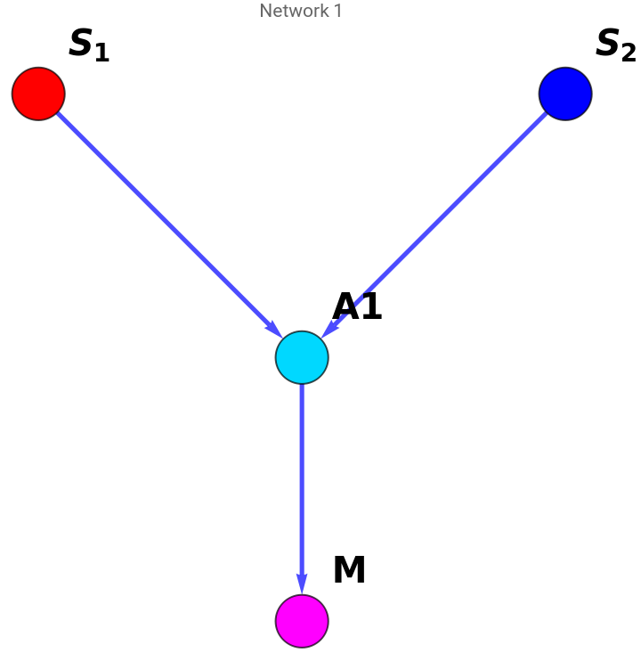
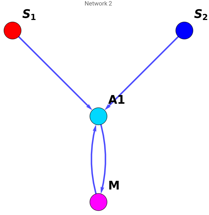
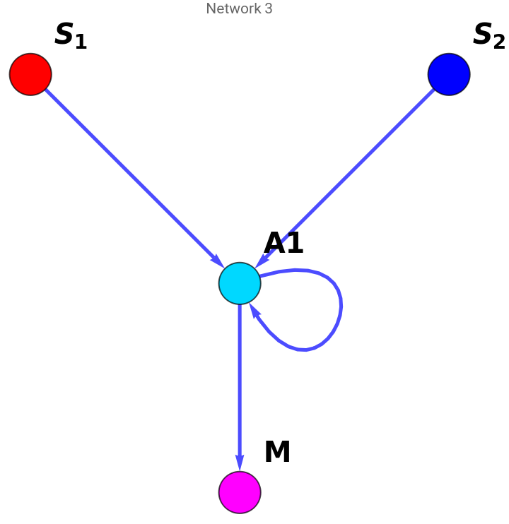
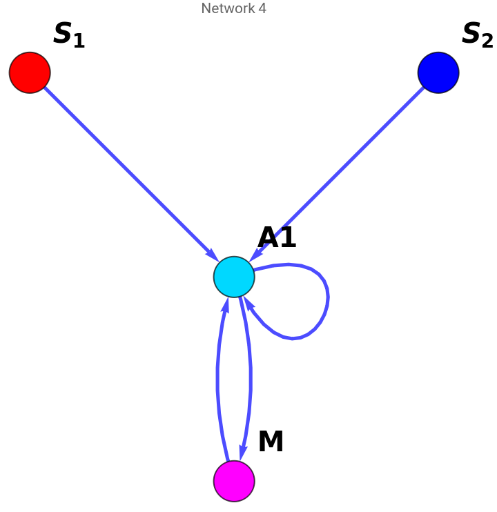
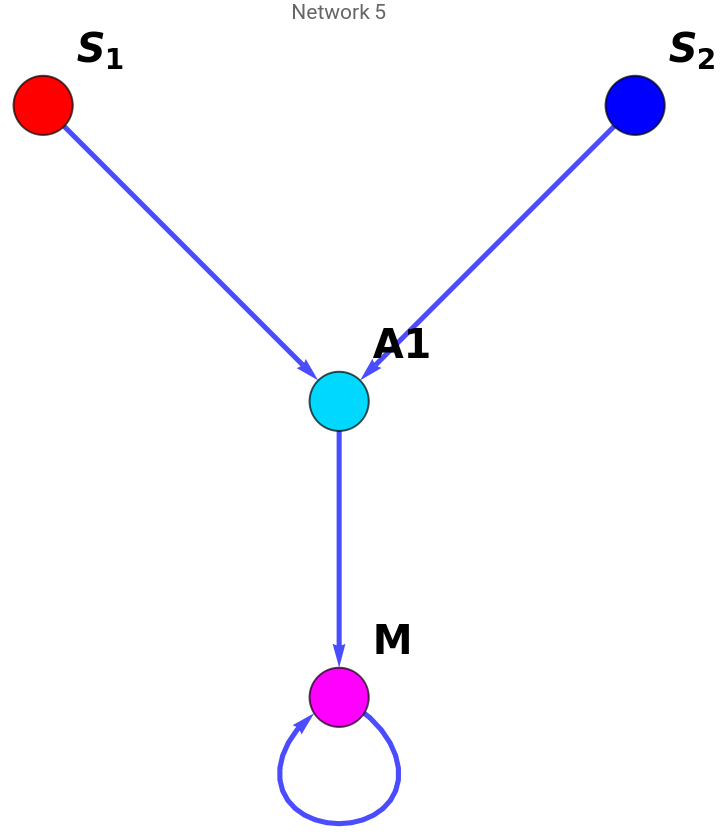
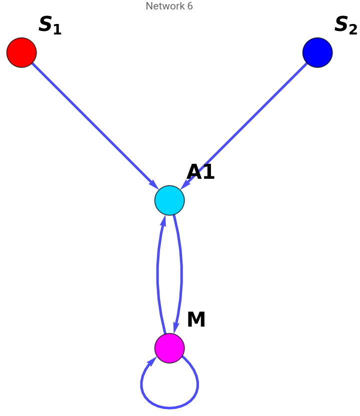
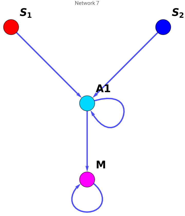
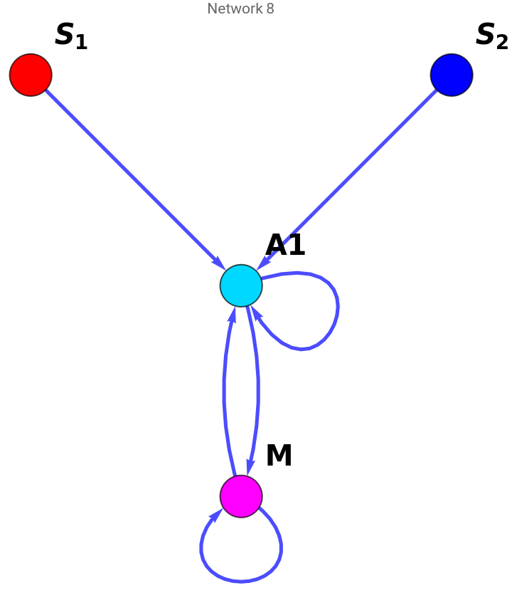
In this part we look at the possible allowed regulation networks for an n node network. In our framework there are two inputs ), one output (M) and at least one intermediate node ). The rule governing the allowed networks are -
1. The inputs and outputs can only interact with each other via the intermediate nodes.
2. Nothing acts on the inputs because they are external to the cell.
3. Both inputs must activate at least one intermediate node.
4. At least one intermediate node must activate the output.
(,
S
1
S
2
(
A
i
1. The inputs and outputs can only interact with each other via the intermediate nodes.
2. Nothing acts on the inputs because they are external to the cell.
3. Both inputs must activate at least one intermediate node.
4. At least one intermediate node must activate the output.
How many edges are allowed for n node network?
How many edges are allowed for n node network?
Given the constraint above, this function evaluates how many maximum possible allowed edges are present in an n node network.
In[]:=
AllowedEdgeCount[nodes_]:=Boole[nodes>3]*(nodes*(nodes-2)-2)+Boole[nodes<=3]*0
In[]:=
AllowedEdgeCount[4]
Out[]=
6
All possible combinations for m edges
All possible combinations for m edges
For a maximum of m edges present in a network, we can extract the possible networks given each edge can be present or absent.
In[]:=
AllPossibleEdgeCombinations[medges_]:=DeleteDuplicates[Table[PadLeft[IntegerDigits[i,2],medges],{i,0,2^medges-1}]]
In[]:=
AllPossibleEdgeCombinations[4]
Out[]=
{{0,0,0,0},{0,0,0,1},{0,0,1,0},{0,0,1,1},{0,1,0,0},{0,1,0,1},{0,1,1,0},{0,1,1,1},{1,0,0,0},{1,0,0,1},{1,0,1,0},{1,0,1,1},{1,1,0,0},{1,1,0,1},{1,1,1,0},{1,1,1,1}}
All possible allowed networks considering connectivity
All possible allowed networks considering connectivity
Given the constraints mentioned above, we can get the set of allowed networks (directed graph) for n nodes in the form of a interaction matrix V where represents interaction from tonode.Innnodes,thefirsttwoelementsarethetwoinputs,thelastelementistheoutputMandtheintermediatenodes lie in between. Value 1/0 represents presence/absence of interaction.
V
ij
th
i
th
j
In[]:=
AllAllowedNetworks[nodes_]:=Module[{mat,adj,nedges,networks,vertexcoord,vertexlabel,vertexstyle,adjtr},mat=ConstantArray[0,{nodes,nodes}];adj=ConstantArray[0,{nodes,nodes}];nedges=AllowedEdgeCount[nodes];Table[mat[[i,nodes]]=i-2,{i,3,nodes}];Table[mat[[i,j]]=nodes-2+(j-3)*nodes+i,{i,1,nodes},{j,3,nodes-1}];networks=AllPossibleEdgeCombinations[nedges];adjtr=DeleteDuplicates@Table[Table[adj[[i,j]]=Boole[IntegerQ@networks[[k,mat[[i,j]]]]]*networks[[k,mat[[i,j]]]],{i,1,nodes},{j,1,nodes}];If[Total[adj[[1]]]*Total[adj[[2]]]*(Total@adj[[;;,nodes]]-adj[[nodes,nodes]])>0,adj],{k,Length@networks}];Delete[adjtr,Position[adjtr,Null]]]
In[]:=
AllAllowedNetworks[4]
Out[]=
{{{0,0,1,0},{0,0,1,0},{0,0,0,1},{0,0,0,0}},{{0,0,1,0},{0,0,1,0},{0,0,0,1},{0,0,1,0}},{{0,0,1,0},{0,0,1,0},{0,0,1,1},{0,0,0,0}},{{0,0,1,0},{0,0,1,0},{0,0,1,1},{0,0,1,0}},{{0,0,1,0},{0,0,1,0},{0,0,0,1},{0,0,0,1}},{{0,0,1,0},{0,0,1,0},{0,0,0,1},{0,0,1,1}},{{0,0,1,0},{0,0,1,0},{0,0,1,1},{0,0,0,1}},{{0,0,1,0},{0,0,1,0},{0,0,1,1},{0,0,1,1}}}
Visualizing all possible allowed networks
Visualizing all possible allowed networks
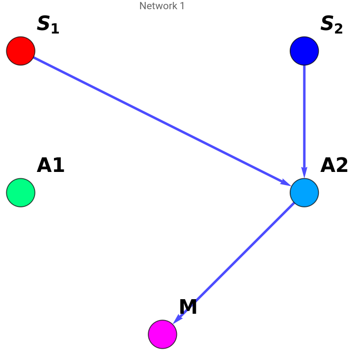
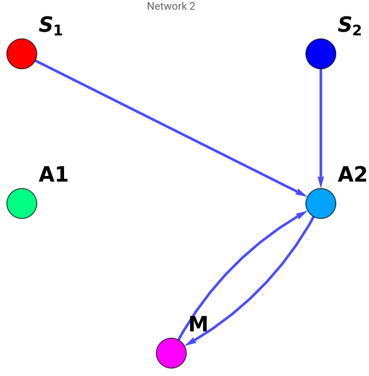
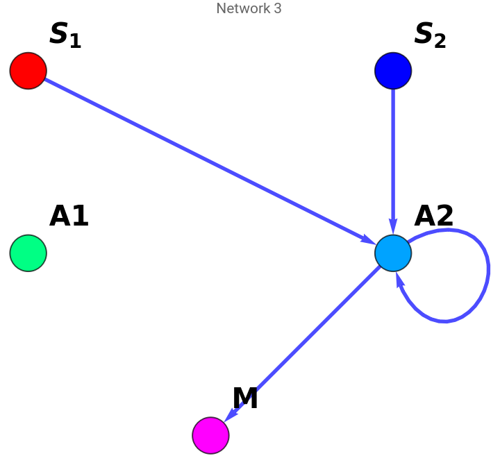
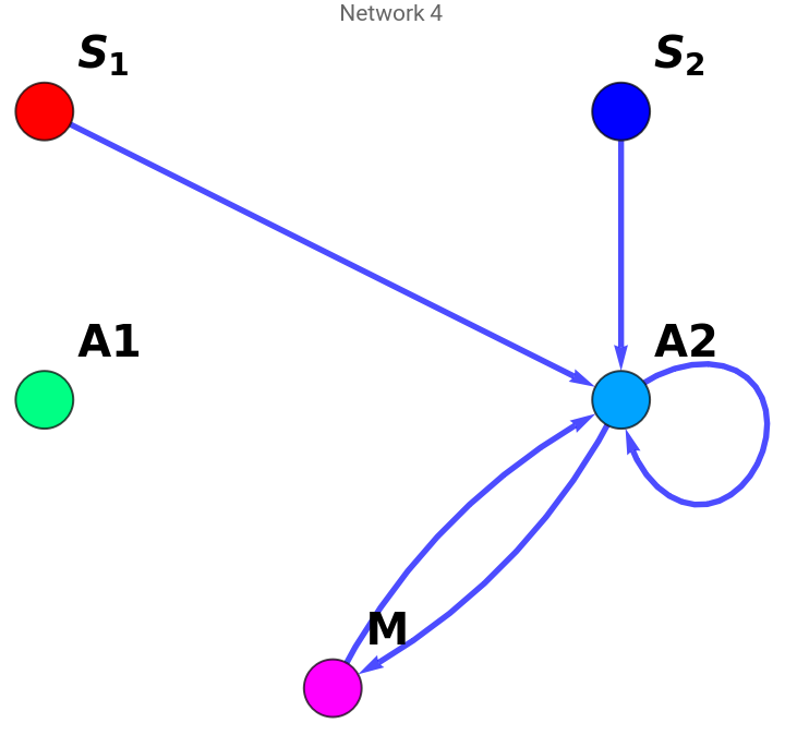
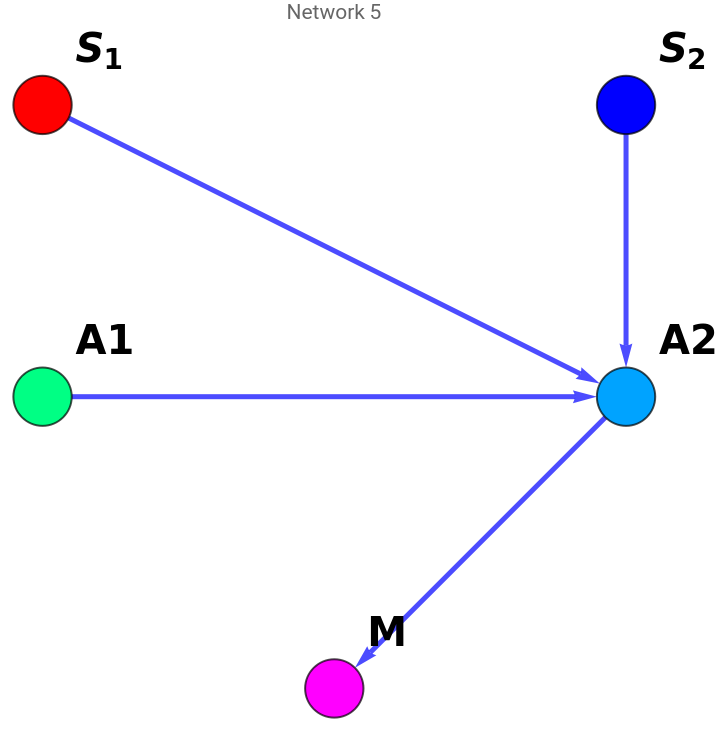
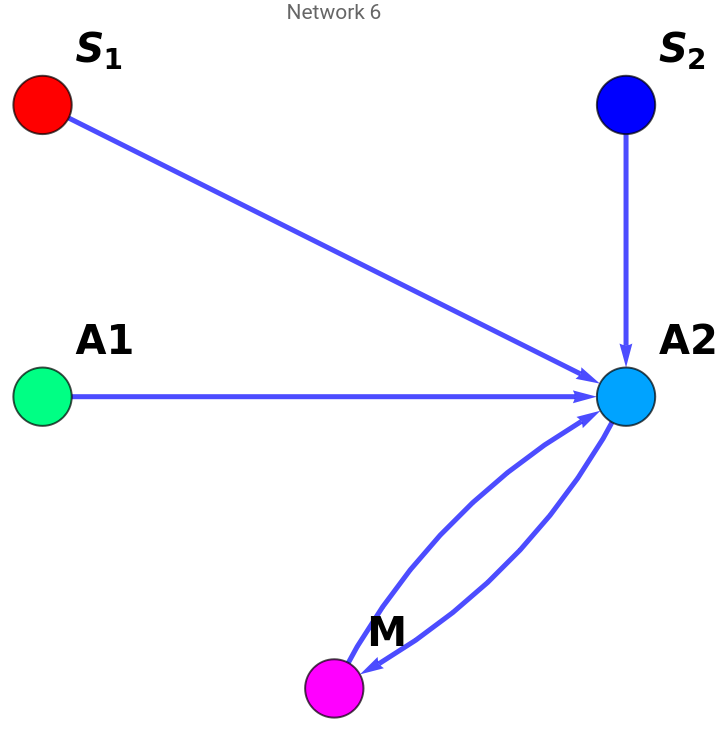
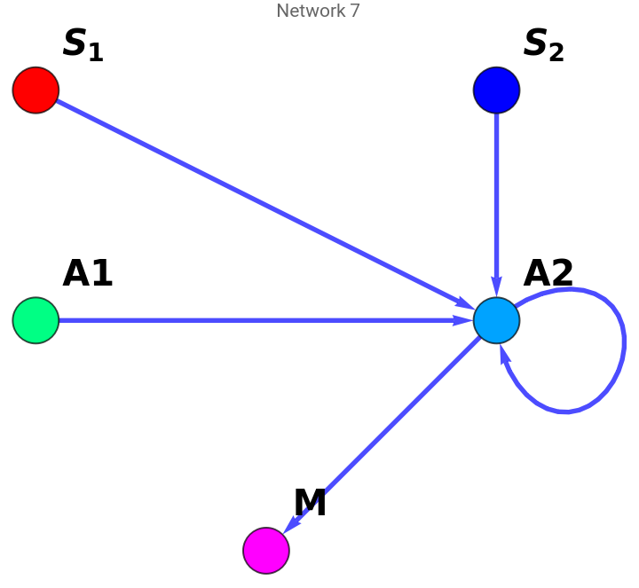
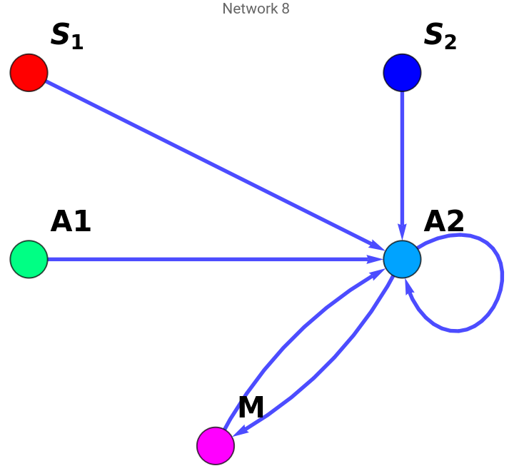
We can visualize all possible allowed networks for n nodes (first input of the function DrawAllowedNetworks) using the function below. For any network having 5 or more nodes has too many possibilities. So the second input of the function DrawAllowedNetworks (numberOfNetworks) restricts the total number of shown networks to numberOfNetworks.
In[]:=
DrawAllowedNetworks[nodes_,numberOfNetworks_]:=Module[{vertexLabelSize,edgeThickness,vertexSize,vertexCoord,vertexLabel,vertexStyle,uniqueNetworks,},vertexLabelSize=20;edgeThickness=0.0075;vertexSize=0.2;vertexCoord=Join[{{-1,2},{1,2}},Table[{-(nodes-4)+2*(i-1),1},{i,nodes-3}],{{0,0}}];vertexLabel=Join[{1->"",2->"",nodes->"M"},Table[i->StringJoin["A",ToString[i-2]],{i,3,nodes-1}]];vertexStyle=Join[{1->Red,2->Blue,nodes->Magenta},Table[i->Hue[0.7*i/nodes],{i,3,nodes-1}]];uniqueNetworks=AllAllowedNetworks[nodes];Table[AdjacencyGraph[uniqueNetworks[[i]],EdgeStyleDirective[Blue,Thickness[edgeThickness]],VertexSizevertexSize,VertexStylevertexStyle,VertexLabelsvertexLabel,VertexLabelStyleDirective[Black,Bold,vertexLabelSize],PlotLabelStringJoin["Network ",ToString@i],VertexCoordinatesvertexCoord],{i,Min[Length@uniqueNetworks,numberOfNetworks]}]]
S
1
S
2
Examples of the function usage -
Four nodes
Four nodes
In[]:=
DrawAllowedNetworks[4,10]
Out[]=
,
,
,
,
,
,
,
Five nodes
Five nodes
Too many possibilities, so number of shown 5 node networks is restricted by the second input.
In[]:=
DrawAllowedNetworks[5,10]
Out[]=
,
,
,
,
,
,
,
,
,
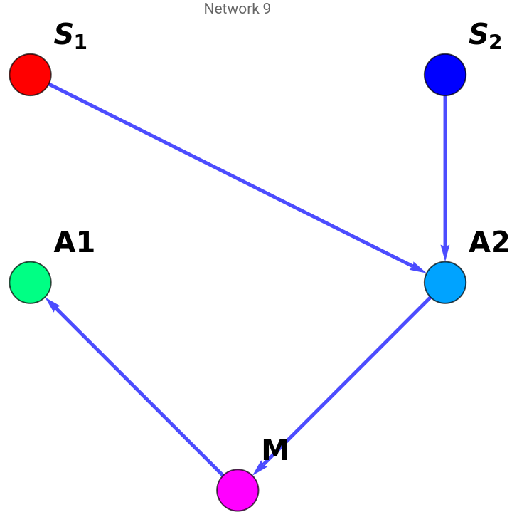
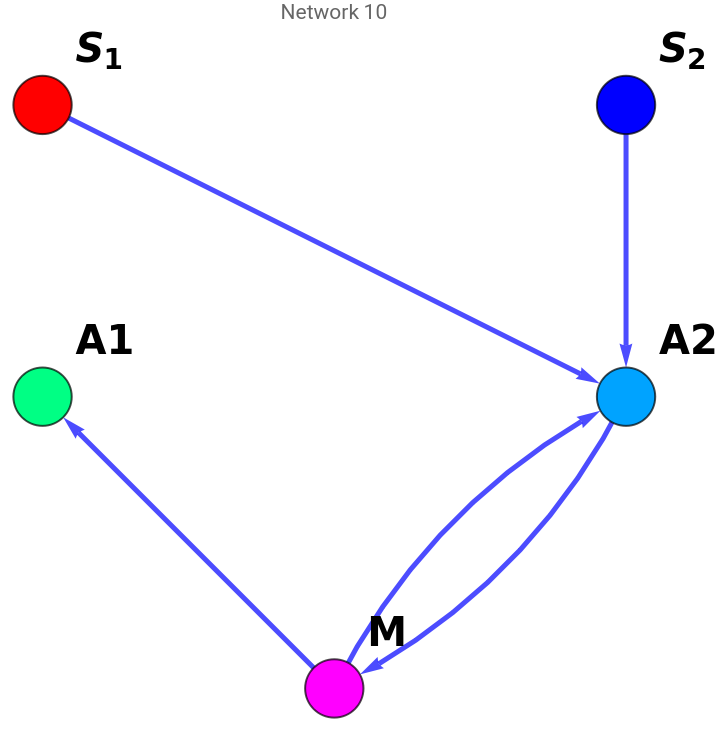
Possible regulation networks for a given connected network
Possible regulation networks for a given connected network
For a given connected network (interaction matrix) it is possible to extract all possible regulation network where each directed edge either corresponds to activation (+1) or repression (-1).
In[]:=
ActivationRepressionNetworks[ConnectedNetwork_]:=Module[{nedges,pos,actrep,matn},matn=ConnectedNetwork;nedges=Total@Total@matn;pos=Position[matn,1];actrep=Table[PadLeft[IntegerDigits[i,2],nedges],{i,0,2^nedges-1}];Table[Table[i=pos[[k,1]];j=pos[[k,2]];matn[[i,j]]=2*actrep[[l,k]]-1,{k,Length@pos}];matn,{l,Length@actrep}]]
Drawing all possible allowed regulation networks
Drawing all possible allowed regulation networks
We can also draw all possible regulation network where Red edge represents repression and Green edge represents activation.
Drawing a single network
Drawing a single network
This function draws a single network using the interaction matrix. Red edge is repression and Green edge is activation.
Solving for steady state output M
Solving for steady state output M
Defining variables for n node network to solve the steady state equations
Defining variables for n node network to solve the steady state equations
To adaptively solve the equation for an n node network we need to define the intermediate nodes for the equation adaptively. Which we are doing in this function.
Solving for M for a given network
Solving for M for a given network
Visualizing input output relationship
Visualizing input output relationship
Drawing network and input output relationship together
Drawing network and input output relationship together
Minimal networks for antagonism
Minimal networks for antagonism
Minimal network showing slope antagonism
Minimal network showing slope antagonism