USA fatalities estimates based on curve fit and SIR model
Resource is various official places, it now becomes clear that the death rate is under reported by as much as 50%
In[]:=
ResourceObject["Epidemic Data for Novel Coronavirus COVID-19"]
Out[]=
ResourceObject


In[]:=
usdeaths=ResourceData["Epidemic Data for Novel Coronavirus COVID-19","WorldCountries"]SelectMatchQ,#Country&[All,"Deaths"];
In[]:=
usd=TimeSeriesWindow[First[usdeaths],{{2020,3,2},{2020,12,30}}]
Out[]=
TimeSeries

In[]:=
usdl=Values[usd];
Number of days data is taken from
In[]:=
ndim=First[Dimensions[usdl]];
In[]:=
58
Out[]=
58
In[]:=
usdlr=Table[usdl[[i]]-usdl[[i-1]],{i,2,ndim,1}];
First date of capture
In[]:=
usd["FirstDate"]
Out[]=
In[]:=
logusd=N[Log[usdl]];
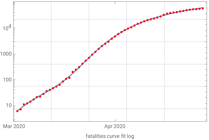
Fatality curve fit model.
Curve fit is made on logarithmic scale - Exponential growth becomes straight line (linear fit)
denominator chosen so total fatalities approach constant value as t-> infinity
Curve fit is made on logarithmic scale - Exponential growth becomes straight line (linear fit)
denominator chosen so total fatalities approach constant value as t-> infinity
In[]:=
model=(a0+a1t+a2t^2+a3t^3+a4t^4)/(1.+a6t^4);
In[]:=
fit=FindFit[logusd,model,{a0,a1,a2,a3,a4,a5,a6},t,MaxIterations200]
Out[]=
{a01.55653,a10.252616,a2-0.00560352,a3-0.000350556,a40.0000458998,a51.,a63.50242×}
-6
10
Total fatalities as t-> infinity:
In[]:=
Exp[a4/a6/.fit]
Out[]=
491472.
In[]:=
p2=DateListLogPlot[usd,PlotStyleRed,JoinedFalse,PlotLegends{"data"}];
In[]:=
p1=DateListLogPlot[TimeSeries[Table[Exp[Evaluate[model/.fit]],{t,1,ndim}],{"March 2,2020"}]];
In[]:=
Show[p1,p2,FrameTrue,GridLinesAutomatic,FrameLabel"fatalities curve fit log"]
Out[]=

In[]:=
p3=ListPlot[usdl,PlotStyleRed,JoinedFalse,PlotLegends{"data"}];
In[]:=
p4=Plot[Evaluate[Exp[model]/.fit],{t,1,ndim}];
In[]:=
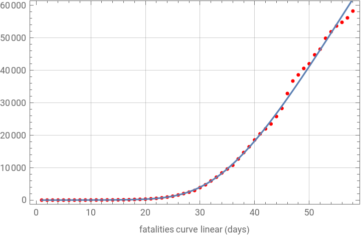
Show[p3,p4,FrameTrue,GridLinesAutomatic,FrameLabel"fatalities curve linear (days)"]
Out[]=
In[]:=
g[t_]:=Exp[(a0+a1t+a2t^2+a3t^3+a4t^4)/(1.+a6t^4)]/.fit
In[]:=
Table[g'[i],{i,ndim}]'
Out[]=
′
{1.45974,1.74254,2.0417,2.35518,2.68632,3.04677,3.45953,3.96184,4.60865,5.477,6.67252,8.33936,10.6745,13.9476,18.5267,24.9077,33.7457,45.8803,62.3459,84.3571,113.256,150.42,197.133,254.436,322.985,402.94,493.908,594.953,704.664,821.274,942.795,1067.16,1192.37,1316.54,1438.05,1555.52,1667.83,1774.16,1873.91,1966.72,2052.42,2130.96,2202.45,2267.07,2325.09,2376.81,2422.57,2462.72,2497.62,2527.64,2553.11,2574.39,2591.8,2605.63,2616.2,2623.75,2628.55,2630.84}
Guessing two important parameters gamma= expected infectious duration ( days) and alpha=case fatality rate (not used)
In[]:=
gamma=1/10.5alpha=.01
Out[]=
0.0952381
Out[]=
0.01
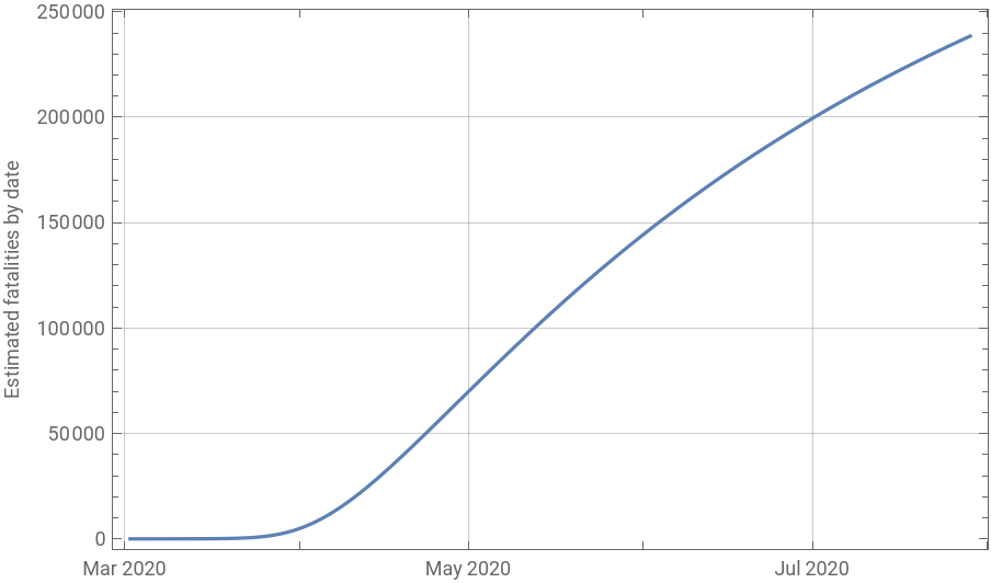
Estimate fatalities into future months
In[]:=
idata=Table[g[i],{i,2.6*ndim}];
In[]:=
infected=TimeSeries[idata,{"March 2,2020"}]
Out[]=
TimeSeries

In[]:=
DateListPlot[infected,FrameTrue,GridLinesAutomatic,FrameLabel"Estimated fatalities by date"]
Out[]=
Estimate daily fatalities (derivative of total fatalities) and compare to data taken.
In[]:=
drate=TimeSeries[Table[g'[i],{i,1.9*ndim}],{"March 2,2020"}]
Out[]=
TimeSeries

In[]:=
d1=DateListPlot[drate,PlotRange{0,5000}];
In[]:=
d2=DateListPlot[TimeSeries[usdlr,{"March 3,2020",Automatic,1}],PlotStyleRed,JoinedFalse,PlotLegends{"data"},GridLinesAutomatic];
In[]:=
Show[d1,d2,FrameTrue,GridLinesAutomatic,FrameLabel"Estimated daily fatalities"]
Out[]=
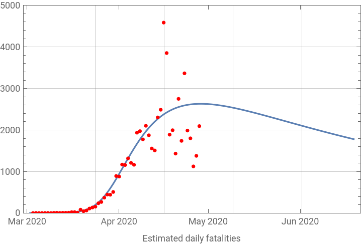
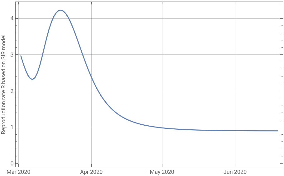
As can be seen from other countries, the daily fatalities do not drop rapidly as one would expect from a standard SIR model when herd immunity has been reached, but rather reach a plateau. The plateau happens because we are not near herd immunity yet but we managed to control spread with social distancing. If we assume that the reproduction rate R is not a constant but dependent on behaviour (and perhaps weather) in an SIR model and assume we are still far from her immunity then we can estimate R(t) from the model and curve fit:
In[]:=
bmg=TimeSeries[Table[g''[i]/g'[i]/gamma+1.,{i,1.9*ndim}],{"March 2,2020"}];
In[]:=
DateListPlot[bmg,FrameTrue,GridLinesAutomatic,FrameLabel"Reproduction rate R based on SIR model"]
Out[]=
Conclusion
Conclusion
We started out with a reproduction rate of about 3. Initial attempts of contact tracing reduced R down to about 2.3 but failed and the reproduction rate rose to about 4.2 mid March. Social distancing then gradually reduced R down to about 1 today. Keeping the current social distancing in place, R fill fall slightly below 1 by the end of June.
Assume data and model are correct, we will have 200,000 fatalities by independence day. Recent news suggest that the data under reports - this would raise the estimated outcome.
Assume data and model are correct, we will have 200,000 fatalities by independence day. Recent news suggest that the data under reports - this would raise the estimated outcome.