ABSTRACT (original article): We present the solution of six problems drawn from the chemical engineering and applied mathematics fields of study. These problems are solved using the arc-length continuation method. Among a large number of examples, we have chosen to treat the following case studies because they illustrate basic concepts such as solution multiplicity when dealing with systems of nonlinear algebraic equations or boundary value problems: 1) Plotting an ∞-shaped curve called the Bernoulli’s Lemniscate; 2) Computing the Joule-Thomson inversion curve for a pure gas using the Soave-Redlich-Kwong cubic equation of state; 3) Predicting the Compressibility Factor and Molar Volume versus the Reduced Temperature; 4) Determining region where steady-state multiplicity is observed in a continuous stirred-tank reactor (CSTR) with multiple reactions and heat effects; 5) Finding the steady-state temperature and conversion of a Propylene Glycol Reactor; and 6) Investigating the Frank–Kamenetskii problem arising in the self-heating of a reactive solid. Reader should be advised that problem 1 may seem slightly mathematical in nature. However, case studies 2–6 could be very useful to instructors involved in teaching not only numerical methods but also chemical thermodynamics and chemical reaction engineering. For one of the above listed case studies, we unveil the MATLAB© code, that we have employed, in the Appendix. In addition, we will emphasize on the versatility of this mathematical software through the extensive usage of the built-in command fsolve, for the presently undertaken computations. Finally, we conclude this paper by sharing our experience teaching this subject to graduate students at King Fahd University of Petroleum & Minerals. CITATION (original article): U. Al-Mubaiyedh and H. Binous, Teaching arc-length continuation in the chemical engineering graduate program using MATLAB©, Comput Appl Eng Educ. 2018; 26: 1033–1049. DOI: https://doi.org/10.1002/cae.21954
Consider a continuous stirred-tank reactor (CSTR) with heat effects and multiple reactions: . Part 1:We find the steady states using both the mass and energy balance equations using Wagon’s method (see Ref. 1). When one chooses =298 and , up to five steady states can be obtained. However, you can select other values for these two parameters and find either a unique steady-state or three steady-states.
ABC
k
1
→
k
2
→
T
0
β=Fρ+UA=298
C
P
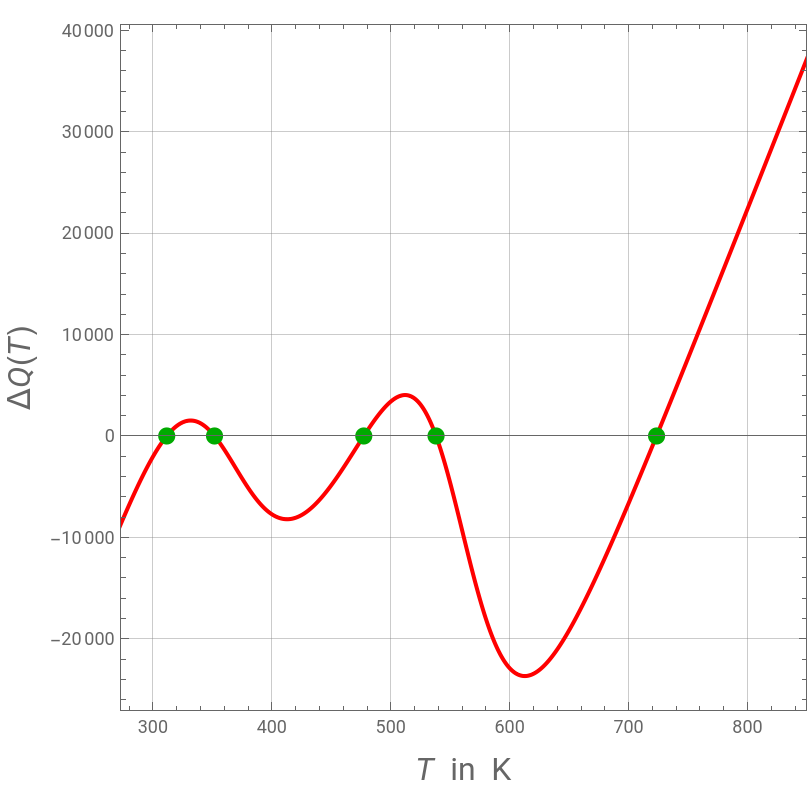
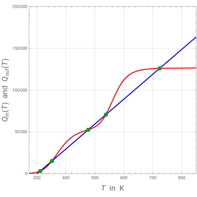
Part 2:We find the steady-states using arc-length continuation using as a continuation parameter and in particular we findthe same five steady-states as in Part 1 when . For details, readers are directed to Ref. 2.Only species is fed to the reactor with an inlet concentration equal to =1.The mass balance equations for the species and are:(T)=/(1+(T)τ),(T)=(T)τ(T)/(1+(T)τ),where is the residence time and (T) and (T) are the reaction rate constants given by the Arrhenius law.The energy balance can be written as (T)=(T),where (T)=-ΔV(T)(T)-ΔV(T)(T),and (T)=FρT-F+UAT-.where and are the heat of reactions, is the molar flow rate, is the heat capacity, is the density, the subscript indicates inlet conditions, and are the overall heat transfer coefficient and the area of the cooling jacket, respectively, =278K is the temperature of cooling, and is the reactor’s volume.The two heat quantities (T) and (T) are plotted versus in red and blue; (T) is a simple linear function (shown by the blue line).The steady states are shown by the green dots in two different plots: (1) (T) and (T) versus ; and (2) (T)-(T)=ΔQ(T).
β=Fρ+UA
C
P
β=298
A
C
A0
A
B
C
A
C
A0
k
1
C
B
k
1
C
A
k
2
τ
k
1
k
2
Q
in
Q
out
Q
in
H
1
k
1
C
A
H
2
k
2
C
B
Q
out
C
P
ρ
0
C
P,0
T
0
T
j
Δ
H
1
Δ
H
2
F
C
P
ρ
0
U
A
T
j
V
Q
in
Q
out
T
Q
out
Q
in
Q
out
T
Q
out
Q
in
After work by: Mike Gordon (University of California Santa Barbara)
Problem’s data
Inlet concentration of A:
Ca0=1;
Heat of reactions:
dH1=-55000;dH2=-71500;
Inlet temperature:
T0=298;
Coefficients for computing Qout:
A1=298;B1=300;C1=1;
Reactor’s time constant:
tau=0.01;
Reactor’s volume:
V=0.01;
Cooling temperature:
Tj=278;
Rate constants:
k1[T_]:=3.3*Exp[-9900/1.987*(1/T-1/300)];k2[T_]:=4.58*Exp[-27000/1.987*(1/T-1/500)];
Steady-state concentrations:
Ca[T_]:=Ca0/(k1[T]*tau+1);Cb[T_]:=k1[T]*tau*Ca[T]/(k2[T]*tau+1);Cc[T_]:=k2[T]*tau*Cb[T];
Heat inlet and outlet:
Qin[T_]:=V*(-k1[T]*dH1*Ca[T]-k2[T]*dH2*Cb[T]);Qout[T_]:=A1T-B1T0-C1Tj;
Used for the table given below:
labels=Table[i,{i,1,5}];
Part 1 : solution using Wagon’s method
Part 1 : solution using Wagon’s method
Q
in
Q
out
In[]:=
plt1=Plot[{Qin[T],Qout[T]},{T,250,850},FrameTrue,FrameLabel{Style[Row[{Style["T",Italic]," in K"}],16],Style[Row[{,"(",Style["T",Italic],") and ",,"(",Style["T",Italic],")"}],16]},PlotStyle{Red,Blue},ImageSize.9×450{1,1},AspectRatio1,GridLinesAutomatic,FrameTrue,PlotRange{{273,850},{0,200000}},AxesOrigin{273,0}];(*(T)and(T)versusT*)
Style["Q",Italic]
"in"
Style["Q",Italic]
"out"
Q
in
Q
out
Q
out
Q
in
In[]:=
plt2=Plot[Qout[T]-Qin[T],{T,250,850},FrameTrue,FrameLabel{Style[Row[{Style["T",Italic]," in K"}],16],Style[Row[{"Δ",TraditionalForm[Q[T]]}],16]},PlotStyle{Red},ImageSize.9×450{1,1},AspectRatio1,GridLinesAutomatic,FrameTrue,PlotRange{{273,850},All},AxesOrigin{273,0},PlotPoints1000];(*(T)-(T)=ΔQ(T)versusT*)
Q
out
Q
in
steady-states can be obtained using Wagon’s approach (see Ref. 1 for details)
In[]:=
tbl=First[Cases[plt2,x_LineFirst@x,Infinity]];tbl2=Table[tbl[[i,1]],{i,1,Length[tbl]}];signs=Sign[Map[Qout,tbl2]-Map[Qin,tbl2]];signs2=Rest[signs]*Rest[RotateRight[signs]];posns=Position[signs2,-1];seeds=tbl2[[Flatten[posns]]];root[xseed_]:=FindRoot[Qin[x]Qout[x],{x,xseed}]//Quiet;solns=root/@seeds//Chop;(*Wagon'smethodforsteady-statesdetermination*)
Superimposed are (T)-(T)=ΔQ(T)versusT and the five steady-states
Q
out
Q
in
In[]:=
Show[plt2,Graphics[{Darker@Green,PointSize[0.025],Point[{x,Qout[x]-Qin[x]}]/.solns}]](*upto5steady-statesarefoundanddepictedbythegreendots*)
Out[]=
Superimposed are (T)and(T)versusT and the five steady-states
Q
in
Q
out
In[]:=
Show[plt1,Graphics[{Darker@Green,PointSize[0.025],Point[{x,Qin[x]}]/.solns}]](*upto5steady-statesarefoundanddepictedbythegreendots*)
Out[]=
References
References
◼
[1] S. Wagon, Mathematica® in Action: Problem Solving through Visualization and Computation, 3rd ed., Berlin: Springer-Verlag, 2010.
◼
[2] U. Al-Mubaiyedh and H. Binous, Teaching arc-length continuation in the chemical engineering graduate program using MATLAB©, Comput Appl Eng Educ. 2018; 26: 1033–1049. https://doi.org/10.1002/cae.21954
CITE THIS NOTEBOOK
CITE THIS NOTEBOOK
Multiple reactions in a continuous stirred-tank reactor with heat effects
by Housam Binous & Ahmed Bellagi
Wolfram Community, STAFF PICKS, December 20, 2024
https://community.wolfram.com/groups/-/m/t/3342664
by Housam Binous & Ahmed Bellagi
Wolfram Community, STAFF PICKS, December 20, 2024
https://community.wolfram.com/groups/-/m/t/3342664