Goal: The goal of this project is to construct a quantum version of the cellular automata model for fluid flow discussed in “A New Kind of Science”. This will be done by considering all the possible outgoing directions in the collision between particles that conserve momentum. The starting point will be the hexagonal lattice. The properties of the micro-states and macro-states will be studied and compared with the “classical” model. Of interest is whether the Navier-Stokes equation describes the macroscopic behaviour of this model and the ways in which the “multiway graph” will behave .
Results: The simulations of three types of systems were accomplished: closed systems, open systems with periodic boundary conditions, and tubes in which the fluids were propagated. Three types of multiway graphs were observed: cyclic , tree-like and clustered graphs, the first one was associated with trivial cycles and the last two were associated with ‘random’ states. Causal invariance was only observed in the trivial ordered states. Additionally, a the states were analyzed from a macroscopic perspective by dividing the systems in bigger sections and averaging its properties (number of particles and linear momentum). By analyzing different pathways within the multiway graphs, it was observed that different branches shared similar macroscopic behaviour.
Future work: There is still a lot to explore in the fluid systems conformed by the rules specified above. Simulations with larger number of particles is of great interest to study the continuum limit, which can be compared with results obtained from Navier-Stokes equations.
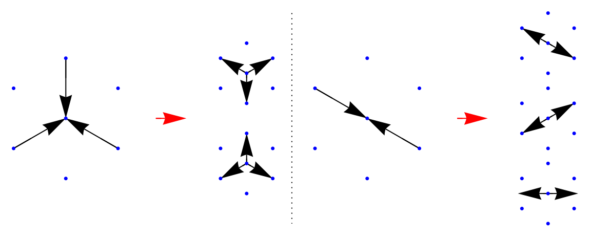
In his book A New Kind of , Stephen Wolfram studies fluid flow considering a set of discrete particles in an hexagonal lattice. These particles would move in a straight line within the lattice, but when they collide with other particles, the outcome of these collisions follow a deterministic set of rules. Here, we considered all possible outcomes in collisions that conserve the total number of particles and linear momentum. In our model, all particles same velocity of the particles is constant, which preserves kinetic energy in collisions. Whenever we have there are 2 (3) outcomes for 3 (2) head-to-head particle collisions respectively as shown in the diagram below.
1
Science
Gas in a box
Gas in a box
We begin with simple systems!
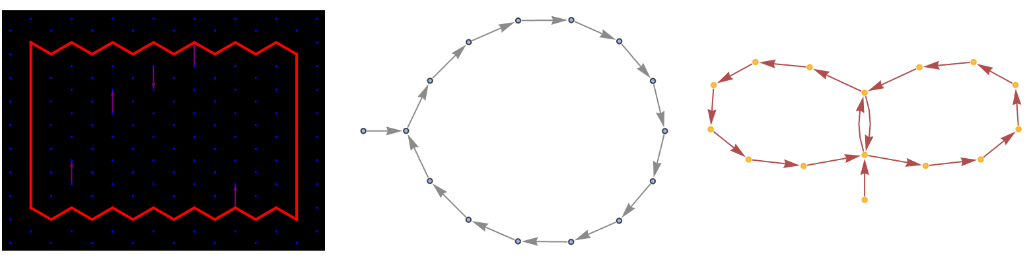
From this systems, cyclic multiway and causal graphs are expected, since the state repeats with a determined period. This system is causal invariant and we expected it be since the system is a cycle with a 14 time-step cycle.
Let’s randomize the initial state!
Let’s randomize the initial state!
This system will have many conflicting collisions and will create branches as a consequence. We can observe how this type of systems have a large number of possible outcomes very fast.
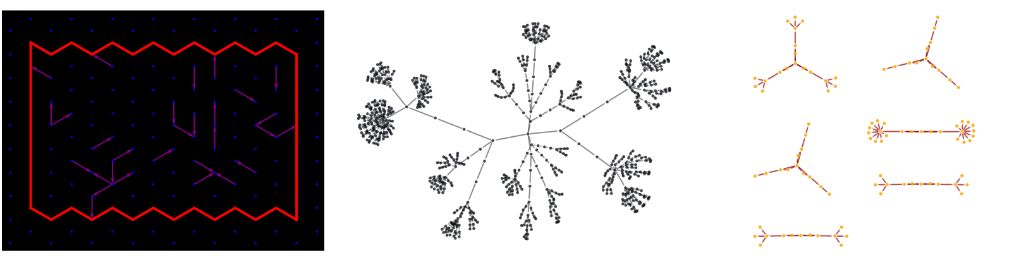
The six separated causal graphs shown above tell us that each of the initial six branches shown in the graphs above develop independently of each other. In other words, we start our time evolution at one of the six possible states available after the first time-step, the states in the other branches wouldn’t be in the set of possible states.
What if we fill the box?
What if we fill the box?
When we have a larger density, the mean free-path is smaller, more collisions take place and the length of each branch is smaller. We can see how practically at every time step multiple outcomes are possible.
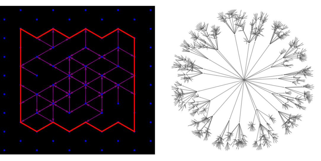
What if we look from far away?
What if we look from far away?
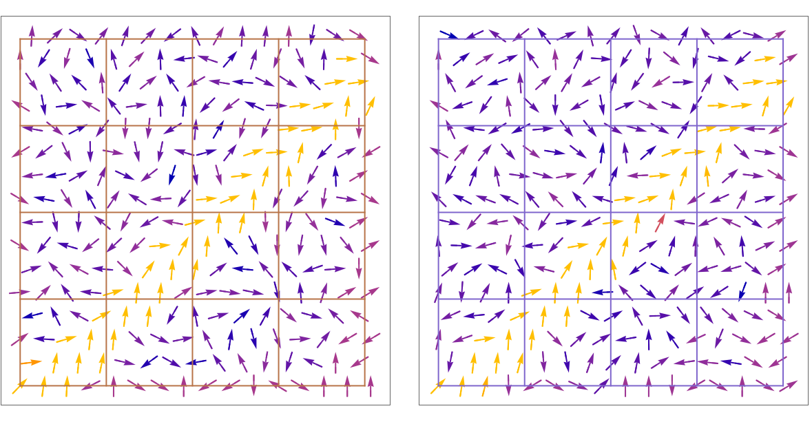
Now we consider a large system and study the macroscopic properties by dividing the box in 16 squares.
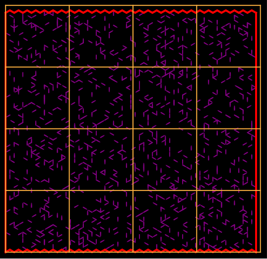
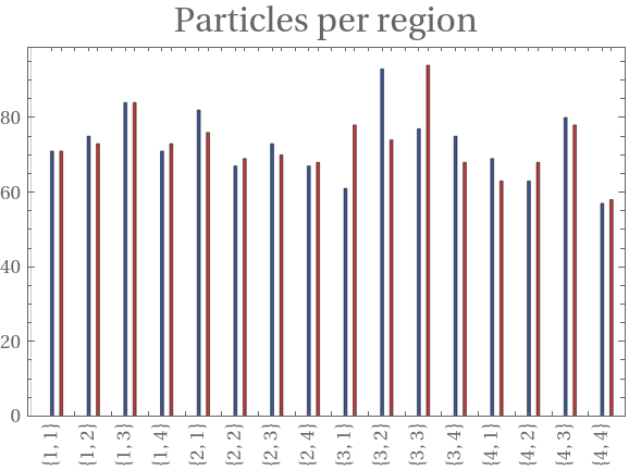
We analyze each square as a whole in two of the possible states after 50 time steps. The figures below show that we number of particles per regions doesn’t vary within the states considered. However, the direction of the total momentum isn’t very aligned.
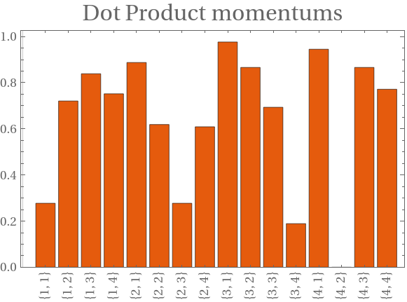
We use the ListVectorPlot to interpolates the flow of the particles and see wether the momentum is in different directions. If we see the box {4,2} (the first number represent the column and the second one the row) we observe than the momentum in box {4,2} varies between the two states.
Open Systems
Open Systems
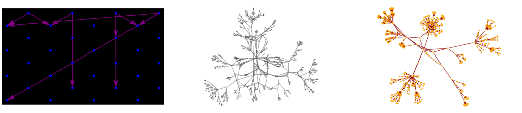
We also take a look into a small system with periodic boundary conditions. We observe a more connected multiway graph, compared to the closed systems, but wether this could be a cause due to the small sample of the systems considered.
Out[]=
Fluid flow
Fluid flow
Step-like tube
Step-like tube
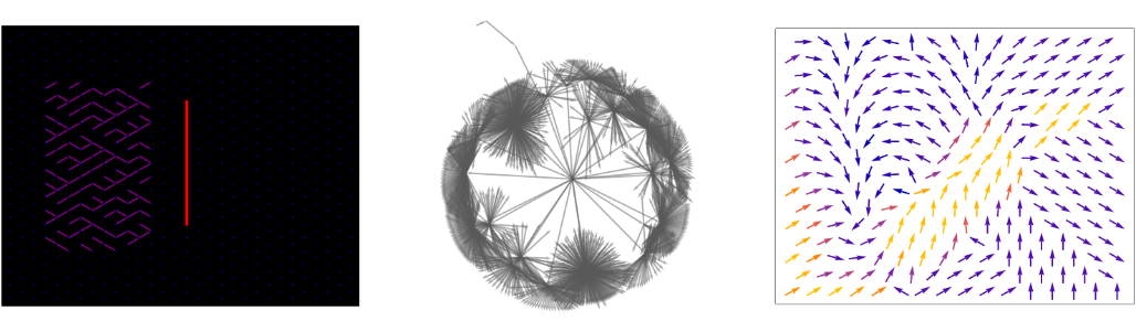
Fluid flow is constructed by setting the system with a total momentum to the right. The multigraph for the first 15 time-steps of this system is shown below. We observe a long tail due to the initial conditions avoid conflicting collisions at the beginning. The image on the right represent the interpolation of the particle’s momentum. It is important to keep in mind that no particles enter the step, this is represented in the vector plot by having lower intensity (blue) vectors in this area.

Open system and a barrier
Open system and a barrier
We also consider a stream of particles hitting a wall in an open system with periodic boundary conditions. The multiway system graph shows a long tail which represent the first few time steps before the particles reach the wall. When reflected, these create many conflicting collisions and this creates many branches, as observed in the diagram.
Out[]=