Introduction
Introduction
Round-off error and truncation error are common inherent sources of error in numerical computation. This post shows the computation and visualization of round-off and truncation errors in specific examples.
Round-off error
Round-off error
A round-off error is the difference between a calculated (approximated with finite-precision arithmetic) value and a reference (exact) value. One area whereby this source of error can be a crucial consideration is the computation of Associated Legendre polynomials (ALP) and spherical harmonics (SH) in quantum chemistry applications. The article “Associated Legendre Polynomials and Spherical Harmonics Computation for Chemistry Applications” (Limpanuparb & Milthorpe, 2014), with the objective of developing an algorithm to efficiently and accurately compute these functions, presents the computation and visualization of round-off errors in ALPs and SHs.
Truncation error
Truncation error
A truncation error is the difference between a numerical approximation of a value and the analytical or true value. An example of a truncation error arises from the approximation of an integral by a sum (truncated infinite series). The article “A Remarkable Identity Involving Bessel Functions” (Dominici, Gill & Limpanuparb, 2012) presents and proves an identity of Bessel function integrals and sums and demonstrates the computation and visualization of truncation errors in the identity.
Computation and visualization
Computation and visualization
Round-off error
Round-off error
Definitions of calculated values, reference values and errors
Definitions of calculated values, reference values and errors
◼
Calculated values are computed using an algorithm developed by the authors described in the article. These values are imported for further calculations of errors.
X
cal
◼
Reference values of ALPs are computed using the function [x_] , where x = cosθ, and degree l and order m satisfy the conditions l ≥ 0 and -l ≤ m ≤ l.
X
ref
P
l_,m_
P
l_,m_
(2l+1)(l-m)!
2π(l+m)!
◼
Absolute error andrelativeerrorare defined as follows: = ) = ),0).
ϵ
a
ϵ
r
ϵ
a
max(|-|,-324
log
10
X
cal
X
ref
ϵ
r
minmax-1,-16
log
10
X
cal
X
ref
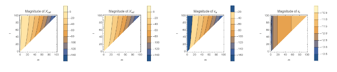
Contour plot of magnitude of errorsExample of evaluation for l ≤ 100 and θ = π100
Contour plot of magnitude of errorsExample of evaluation for l ≤ 100 and θ =
π
100
A list of values is imported (cval1) and values are computed (rval1). The magnitudes of and values are calculated and contained in lists mcval1 and mrval1, respectively.
X
cal
X
ref
X
cal
X
ref
θ=;cval1=Import[NotebookDirectory[]<>"Code/cPlm_100_PI100_0.out","Table"];(*forθ=0*)Length[cval1]-1(*=100*)rval1=Table[N[[Cos[θ]],100],{l,0,100},{m,0,l}];LL=Length[rval1]-1(*=100*)mcval1=Table[If[m≤l,Log10[Abs[cval1〚l+1〛〚m+1〛]]/.{Indeterminate-323}],{l,0,LL},{m,0,LL}];mrval1=Table[If[m≤l,Log10[Abs[rval1〚l+1〛〚m+1〛]]/.{-∞-323}],{l,0,LL},{m,0,LL}];
π
100
X
cal
P
l,m
Out[]=
100
Out[]=
100
The magnitudes of and are computed and contained in lists aepad and repad, respectively.
ϵ
a
ϵ
r
In[]:=
ae=Log10[Abs[cval1-rval1]]/.{Indeterminate-323};ae1=Table[If[m≤l,ae〚l+1〛〚m+1〛],{l,0,LL},{m,0,LL}];re1=Table[Which[m≤l&&rval1〚l+1〛〚m+1〛≠0,Max[Log10[Abs[cval1〚l+1〛〚m+1〛/rval1〚l+1〛〚m+1〛-1]],-16],m≤l,-16,True,],{l,0,LL},{m,0,LL}];
The magnitudes of , , and can be visualized with a contour plot. ListContourPlot is used as an example here. The plots of and magnitudes appear to be identical. This is supported by how and values are all under , as shown in the plots of and magnitudes.
X
cal
X
ref
ϵ
a
ϵ
r
X
cal
X
ref
ϵ
a
ϵ
r
-10
10
ϵ
a
ϵ
r
In[]:=
mcplot=ListContourPlot[mcval1,FrameLabel{m,l},PlotLegendsAutomatic,DataRange{{0,100},{0,100}},PlotLabel->"Magnitude of "];mrplot=ListContourPlot[mrval1,FrameLabel{m,l},PlotLegendsAutomatic,DataRange{{0,100},{0,100}},PlotLabel->"Magnitude of "];aeplot=ListContourPlot[ae1,FrameLabel{m,l},PlotLegendsAutomatic,DataRange{{0,100},{0,100}},PlotLabel->"Magnitude of "];replot=ListContourPlot[re1,FrameLabel{m,l},PlotLegendsAutomatic,DataRange{{0,100},{0,100}},PlotLabel->"Magnitude of "];GraphicsRow[{mcplot,mrplot,aeplot,replot},ImageSize1200]
X
cal
X
ref
ϵ
a
ϵ
r
Out[]=
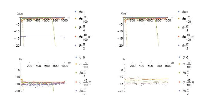
Scatter plot of magnitude of errorsExample of evaluation for l ≤ 1000 and θ = 0,π100,π4,49π100,π2
Scatter plot of magnitude of errorsExample of evaluation for l ≤ 1000 and θ =
0,,,,
π
100
π
4
49π
100
π
2
A list of values is imported (cval2) and values are computed (rval2). The magnitudes of , , and values are calculated and contained in lists mcval2, mrval2, ae2 and re2, respectively.
X
cal
X
ref
X
cal
X
ref
ϵ
a
ϵ
r
cval2=Table[Import[NotebookDirectory[]<>"Code/"<>file,"Table"],{file,{"cPlm_1000_0_0.out","cPlm_1000_PI100_0.out","cPlm_1000_PI4_0.out","cPlm_1000_49PI100_0.out","cPlm_1000_PI2_0.out"}}];rval2=TableN[[Cos[θ]],1000],θ,0,,,,,{l,1000,1000},{m,0,l};mcval2=Table[Log10[Abs[cval2〚i〛〚1〛]]/.{Indeterminate-323},{i,Length[cval2]}];mrval2=Table[Log10[Abs[rval2〚i〛〚1〛]]/.{Indeterminate-323},{i,Length[rval2]}];ae2=Table[Log10[Abs[cval2〚i〛〚1〛-rval2〚i〛〚1〛]]/.{Indeterminate-323},{i,Length[cval2]}];re2=Table[If[rval2〚i〛〚1〛〚m+1〛≠0,Max[Log10[Abs[cval2〚i〛〚1〛〚m+1〛/rval2〚i〛〚1〛〚m+1〛-1]],-16]],{i,Length[cval2]},{m,0,LL}];
P
1000,m
π
100
π
4
49π
100
π
2
The magnitudes of , , and are visualized using ListPlot.
X
cal
X
ref
ϵ
a
ϵ
r
In[]:=
mcplot=ListPlotmcval2,PlotRange{0,-20},PlotLegends"θ=0","θ=","θ=","θ=π","θ=",AxesLabel{m,""},DataRange{0,1000};mrplot=ListPlotmrval2,PlotRange{0,-20},PlotLegends"θ=0","θ=","θ=","θ=π","θ=",AxesLabel{m,""},DataRange{0,1000};aeplot=ListPlotae2,PlotRange{0,-20},PlotLegends"θ=0","θ=","θ=","θ=π","θ=",AxesLabel{m,""},DataRange{0,1000};replot=ListPlotre2,PlotRange{0,-20},PlotLegends"θ=0","θ=","θ=","θ=π","θ=",AxesLabel{m,""},DataRange{0,1000};GraphicsRow[{mcplot,mrplot,aeplot,replot},Spacings->0,ImageSize->1300]
π
100
π
4
49
100
π
2
χ
cal
π
100
π
4
49
100
π
2
χ
ref
π
100
π
4
49
100
π
2
ϵ
a
π
100
π
4
49
100
π
2
ϵ
r
Truncation error
Truncation error
Integral and truncated sum
Integral and truncated sum
The followings are the integral and truncated sum of Bessel functions, respectively.(at)(bt)t = (a,b) = (an)(bn)
∞
∫
0
J
5
2
J
5
2
t
1
5
(|a|)
a
5
2
(|b|)
b
(min(|a|,|b|)
(max(|a|,|b|)
T
N
N
∑
n=1
J
5
2
J
5
2
n
The integral (X; solid) and truncated sum (a,b) (Y; dashed) can be defined and plotted as follows .
T
10
In[]:=
J
l_
1
5
5/2
Min[a,b]
Max[a,b]
π
4
3
4
π
4
10
∑
n=1
J
5
2
J
5
2
n
π
4
3
4
π
4
In[]:=
Z=Union[Y,X];PlotZ,{b,0,2π},PlotStyle{{Darker[Green],Thickness[0.002]},{Darker[Green],Thickness[0.002]},{Darker[Green],Thickness[0.002]},{RGBColor[1,0,0],Thickness[0.0015],Dashed},{RGBColor[1,0,0],Thickness[0.0015],Dashed},{RGBColor[1,0,0],Thickness[0.0015],Dashed},{RGBColor[0,0,1],Thickness[0.0015],DotDashed},{RGBColor[0,0,1],Thickness[0.0015],DotDashed},{RGBColor[0,0,1],Thickness[0.0015],DotDashed}},PlotRange{0,.2},AxesLabel{b,""},PrologText[Style["a",FontSize9,Italic],{1.6,0.04},{-1,0}],TextStyle"=",FontSize9,{1.75,0.039},{-1,0},Text[Style["a",FontSize9,Italic],{2.5,.07},{-1,0}],TextStyle"=",FontSize9,{2.65,.07},{-1,0},Text[Style["a",FontSize9,Italic],{3.1,.12},{-1,0}],TextStyle"=",FontSize9,{3.25,.12},{-1,0},Ticks,,,,,,,,Automatic
π
4
2π
4
3π
4
π
4
2π
4
3π
4
4π
4
5π
4
6π
4
7π
4
8π
4
Visualization of error
Visualization of error