The Wolfram Emerging Leaders Program is a 4 month long project based program designed for gifted high school students to take a deep dive into a topic of their choice. Students work remotely in small groups to take their project from ideation to completion, with the guidance of Wolfram experts. Wolfram Emerging Leaders Program participants are selected from the Wolfram High School Summer Camp, which is open to talented, STEM oriented students age 17 and under.
This essay was written by:
This essay was written by:
Introduction
Introduction
This project aims to explore the propagation of sound in three dimensional regions. We begin by experimenting with acoustic modeling using primitive shapes.
After coming up with a working acoustic model, we utilized a depth sensing neural network to extrapolate data from single images. Using this data, we were able to create a boolean region that is representative of the environment being surveyed.
We integrated this depth map with our acoustic model to obtain attenuation coefficients which were applied to sample audio.
Throughout the process, we were able to come across interesting visualizations, learn about the basic physics behind acoustics and explore digital signal processing.
2D Modeling
2D Modeling
The Helmholtz Equation
The Helmholtz Equation
This partial differential equation is a time independent form of the Wave Equation and is used in physics to model many phenomena. We use it hear to model the pressure distribution in a region when different frequencies are emitted from a monopole sound source.
Preliminary Functions & Attributes from PDE Models Documentation
In[]:=
MaxGridSize[c_,ω_,Resolution_]:=Module[{λ},λ=2 π c/ω;λ/Resolution]Options[AcousticsOptions]={"Resolution"12};AcousticsOptions[c_,ω_,opts:OptionsPattern[]]:=Sequence[Method{"PDEDiscretization"{"FiniteElement","MeshOptions"{"MaxCellMeasure"{"Length"MaxGridSize[c,ω,OptionValue["Resolution"]]}}}}]RegularizedDelta[γ_,X_List,Xs_List]:=Piecewise[{{Times@@Thread[1/(4 γ) (1+Cos[π/(2 γ) (X-Xs)])],And@@Thread[RealAbs[X-Xs]≤2 γ]},{0,True}}]=QuantityMagnitude[ThermodynamicData["Air","SoundSpeed"]];=QuantityMagnitude[ThermodynamicData["Air","Density"]];h[ω_] := MaxGridSize[, ω, 12]=1;Q[ω_, X_List, Xs_List] := RegularizedDelta[h[ω]/2, X, Xs]*; (*ClearAll[AcousticModel]*)AcousticModel[p_,X_List,ρ_,{Q_,F_}]:=Module[{a,factor},factor=-1/ρ*IdentityMatrix[Length[X]];a=PiecewiseExpand[Piecewise[{{factor,True}}]];Inactive[Div][a.Inactive[Grad][p,X],X]-Inactive[Div][F/ρ,X]-Q]
c
air
ρ
air
c
air
Q
Q
Creating The Simulation Domain
In[]:=
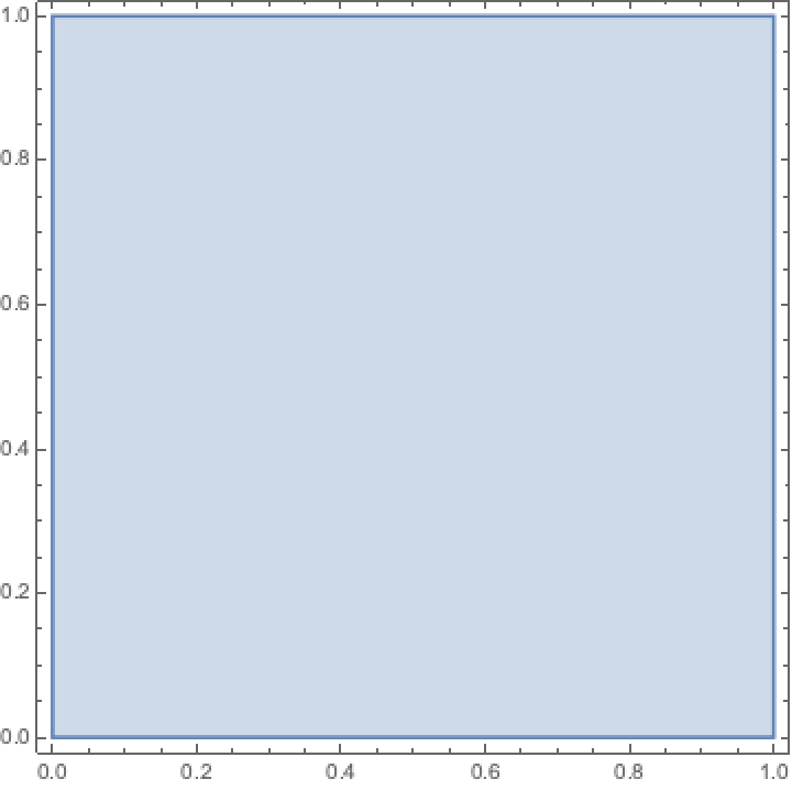
r=1;Ω=Rectangle[{0,0},{r,r}];RegionPlot[Ω]
Out[]=
Setting Sound Source Location
In[]:=
xs=0.5;ys=0.5;r=1;
Creating the Acoustic Model
Creating the Acoustic Model
In[]:=
monopoleModel2D=AcousticModel[p[x,y],{x,y},ρ,{Q[ω,{x,y},{xs,ys}],{0}}]-p[x,y]
2
ω
ρ
2
c
Out[]=
-p[x,y]ρ-
+·-,0,0,-.p[x,y]-·{0}
2
ω
2
c
|
∇
{x,y}
1
ρ
1
ρ
∇
{x,y}
∇
{x,y}
Setting a Boundary Condition
Setting a Boundary Condition
In[]:=
Γ
abcf
ω
c
1
2r
ρ
Creating the PDE
Creating the PDE
In[]:=
pde={monopoleModel2D}/.{c,ρ};
Γ
abcf
c
air
ρ
air
Solving the PDE
Solving the PDE
In[]:=
pfunMonopole2D=ParametricNDSolveValue[pde,p,{x,y}∈Ω,{ω},AcousticsOptions[,ω]]
c
air
Out[]=
ParametricFunction


Visualizing the Results
Visualizing the Results
In[]:=
pMonopole500Hz=pfunMonopole2D[2πf/.{f500}]
InterpolatingFunction

Some examples
Some examples
In[]:=
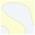
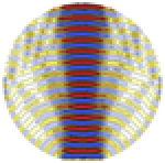
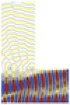
These are plots of the pressure distributions of various regions that we simulated sound propagation in. Each exhibited different characteristics and provided insight on how we can tune our model.
3D Modeling with Primitive Shapes
3D Modeling with Primitive Shapes
The Helmholtz Equation
The Helmholtz Equation
Creating the Simulation Domain
Creating the Simulation Domain
In[]:=
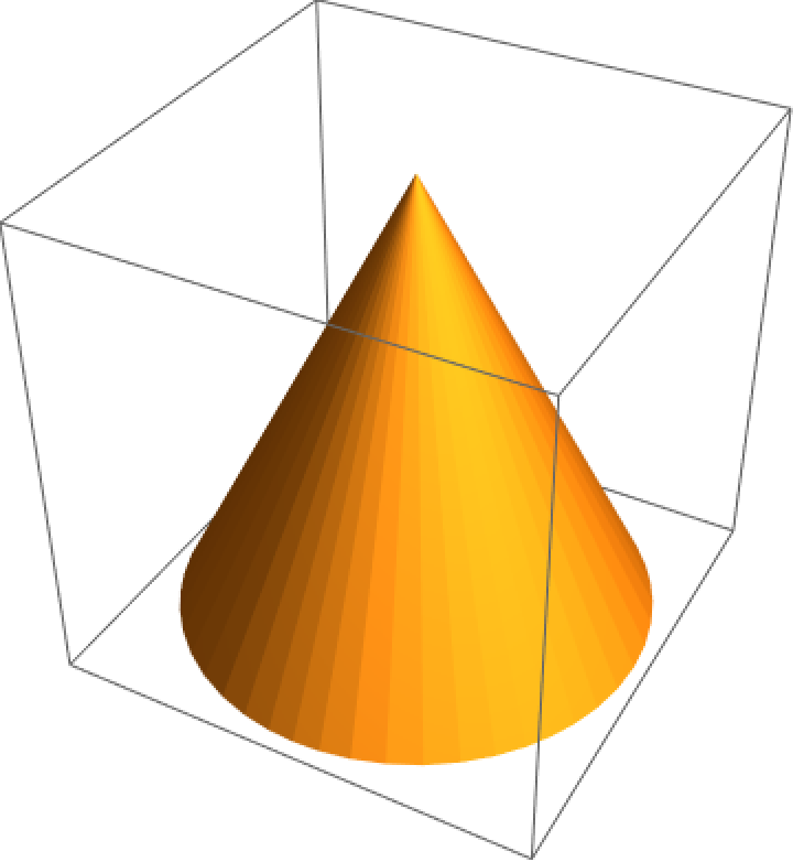
Ω=Region[Cone[{{0,0,0},{0,0,2}},1]];RegionPlot3D[Ω]
Out[]=
Setting Sound Source Location
Setting Sound Source Location
In[]:=
xs=0;ys=0;zs=0;r=1;
Creating the Acoustic Model
Creating the Acoustic Model
Setting a Boundary Condition
Setting a Boundary Condition
Creating the PDE
Creating the PDE
Solving the PDE
Solving the PDE
Visualizing Results
Visualizing Results
Examples & Tests
Examples & Tests
While we tried to generate visualizations for this, the process was too computationally intensive. In the future, we will attempt to render high quality plots to further investigate this model.
Depth Map
Depth Map
Single-Image Depth Perception Net
Single-Image Depth Perception Net
Here is an example image from Wolfram:
A neural network exists that can convert an image into a depth map that doesn’t require multi-view reconstruction.
We obtain the depth map using the neural network “Single-Image Depth Perception Net Trained on NYU Depth V2 and Depth in the Wild Data”.
This allows us to view the depth in a two dimensional visualization
We can better visualize the depthMap with ListPlot3D, which should give us a 3D rendering of the depth of the image.
Notice that some of the depth data has been inaccurately captured. The distance between the farthest point and the closest point in the image doesn’t appear to be recreated in the depth map. The accuracy of relative positions between the points isn’t maintained.
Fine Tuning the output
Fine Tuning the output
We found that multiplying the created depth map by the square root of itself can sometimes yield a more accurate depth map. An example is listed below.
Sample Image:
Again, we obtain the depthMap using the neural net.
This time, we apply a square root function to the depth values.
Visualizing the plot gives us a smooth and accurate depth perception map.
We’ve incorporated some post-processing to help improve the accuracy of depth perception here.
Creating a Boolean Region
Creating a Boolean Region
Method 1 - Hexahedrons
A depth map can be re-created into a boolean region by converting each depth map point into a hexahedron, where the depth value is associated with the height of each hexahedron.
Obtaining a depth map:
Creating the vertices defining each hexahedron that will create the region:
Creating a Mesh Region with the hexahedrons:
Using this mesh region we were able to accurately translate the depth data from an image to a boolean region. Note that each pixel in the image has a depth value associated with it, which dictated how tall the hexahedron corresponding to that pixel is. We simply combined all of these hexahedrons to create the region shown above. We need our data in this format to be compatible with our acoustic model. In order for the mesh region to be compatible, it needs to fit in a 1 by 1 by 1 region. The function below accomplishes that. We simply rescale the values to fit this constraint.
Method 2 - Discretized Region Plot
The depth map can be interpolated into a function and then discretized as shown below.
Obtaining an Interpolation Function for the data:
Plotting the Region:
Discretizing the region plot:
Method 3 - Piecewise Functions with ParametricRegion/ImplicitRegion
The piecewise method only works with a small amount of points:
Convert the points to a piecewise function:
Create an implicit region of the piecewise function, and then discretize it:
Shortcomings
Despite using a variety of approaches to recreate the depth map from implicit regions, to parametric regions, to Delaunay meshes, we were unable to create a process that worked consistently. We’ve outlined a list of our approaches and problems we ran into for each one:
◼
Hexahedrons - This approach looked promising at first glance, but the NDSolve method, which we needed for the acoustic simulation, needed to discretize the region. Unfortunately, the discretization process does not allow for faces that are in contact, which occurs in our hexahedron approach.
◼
Discretized Region Plot - There are two properties that define any region: the region dimension and the embedding region dimension. The former defines the geometric space the region occupies, which is three in this case. The latter defines how the region is expressed on the computer. Using this approach, the embedding region dimension is two. This most likely happened since we are plotting our three dimensional region on a 2 dimensional image before discretizing the region.
◼
Piecewise Function - This approach aimed to obtain an interpolation function that would be more representative than the function returned using ListInterpolate. We created a piecewise function that associated each pixel with its depth value and used ImplicitRegion to make it into a boolean region. This worked great for small arrays, but failed to compute a region for images.
Examples & Tests
3D Modeling with Possible Depth Maps
3D Modeling with Possible Depth Maps
Using a Representative Depth Map as the Simulation Domain
Using a Representative Depth Map as the Simulation Domain
First, we create the simulation domain.
Then we set the sound source location within the domain - where the sound is coming from.
We then create the acoustic model.
We set a boundary condition:
Then we create and solve the PDE:
Visualizing Results:
Examples & Tests
Similar to the 3D tests, these visualizations were hard to render due to lack of computational power. We looked for ways to optimize the process, but were unable to. In the future, we plan on running these on the cloud or more powerful computers.
Conclusion
Conclusion
Overall we were very pleased with our results. Despite coming across some difficult problems, which we weren’t able to address entirely, we felt that we made decent progress and created a project that at the very least explored a lot of the things we wanted to.
In the future, we hope to optimize our three-dimensional acoustic model and apply it to an audio file so we can hear what it would sound like to be in the simulation domain. We also want to create more insightful visualizations to gain a better understanding about our processes and how we can improve them.
Finally, we want to spend more time looking into converting a depth map into a boolean region that our acoustic model can use as a simulation domain. This was arguably one of the hardest parts of our projects and we hope to make more progress.
Acknowledgements
Acknowledgements
We would like to thank our program coordinator, Rory Foulger, for all the support and guidance we received throughout the semester. We truly felt that we’ve been able to learn and form lasting connections within our group and with other members.