Abstract
Abstract
Weight initialization is an important part of creating neural networks that perform well. While most analysis on neural networks has been done on the performance of trained networks, this project will explore the effect of different initializations of weights on the outputs of untrained networks, outlining relations between weight and output distributions and discovering the optimal initializations (from Normal, Gamma, and Uniform) for different network structures that use different common activation functions. The exploratory nature of the analysis will allow for making inferences but not necessarily definitive conclusions (especially for more complex network structures), but it will be useful for further research on optimizing the training process and determining whether the performance of the untrained network predicts the success of the trained network.
Introduction
Introduction
Neural networks show promise in countless fields, ranging from control mechanisms for autonomous vehicles to the analysis of medical images to models that can outperform top players in games like chess. Inspired by the human brain, their structure is defined by multiple layers of neurons, in which each neuron processes input data from the previous layer, implements some function on the data, and passes on the output data to the next layer. Perhaps the most important part of these models are their weights and biases. Weights multiply inputs, thereby controlling the influence any given part of an input has on the activation of a give-n neuron, and biases are added to this product (allowing each neuron to output a different range of values independently from the input).
This project will examine the influence of weights on the outputs of an untrained neural network. By initializing weights from different types of distributions (these will be thoroughly explained in later sections) and implementing them in neural networks of varying architectures and activation functions, we will outline relations and correlations between the distribution of initialized weights and the output of the untrained neural network.
This project will examine the influence of weights on the outputs of an untrained neural network. By initializing weights from different types of distributions (these will be thoroughly explained in later sections) and implementing them in neural networks of varying architectures and activation functions, we will outline relations and correlations between the distribution of initialized weights and the output of the untrained neural network.
Why Examine Untrained Neural Networks?
Why Examine Untrained Neural Networks?
While untrained neural networks will likely not be practical for real-world classification problems anytime soon, an examination of their behavior is still useful for making improvements on the training process, whether those be to increase efficiency or ensure stability. The other main benefit is that the untrained network represents the most baseline form of a neural network and understanding its behavior can show the intrinsic biases of a given network architecture. Finally, these types of analyses are vital to theoretical research on the behavior of neural networks and will be of great utility to efforts of developing new neural network architectures.
Effect on Training
Effect on Training
The initialization of weights has an unimaginably strong effect on the training process, and that’s what this project is centered on. The training process is simply the network running through data and updating the values of the weights as it learns from mistakes. At first it seems like the initial values of the weights should not have any measurable effect on this; after all, the weights should come to the “correct values” in the end.
However, it’s not that simple: while the changing of one weights would likely have no effect, the shifting of the whole distribution of weights can lead to unforeseen consequences, namely the network entirely losing the ability to learn properly.
This can happen in one of two ways: either the weights are initialized in such a way that they begin to to converge towards a point or couple of points as they are updated in the training process, or the weights are initialized so that they rapidly branch in opposite directions, leading to large updates in their values that cause oscillations during training. The former is a problem known as vanishing gradients or gradient loss, while the latter is known as gradient explosion. This project will be focused primarily on preventing, or at the very least, mitigating these issues.
Different Types of Distributions
Different Types of Distributions
Out[]=
Distribution | Formula | Graph | Description |
Normal | f(x) 1 σ 2π - 2 (x-μ) 2 2 σ e | The normal distribution is the classic probability distribution. It's continuous, centered around its mean, μ, with a standard deviation, σ. | |
Gamma | f(x;α,β) α β α-1 x -βx e Γ(α) | The gamma distribution is another continuous probability distribution with two parameters. Instead of μ and σ, the Gamma distribution works with α, the shape parameter, and β, the rate parameter. Note that both of these parameters must be >0 | |
Uniform | f(x)1/(b-a) | The uniform distribution is yet another continuous distribution, however it differs from both the Normal and Gamma distributions in that all outcomes are equally likely within the range of the function. |
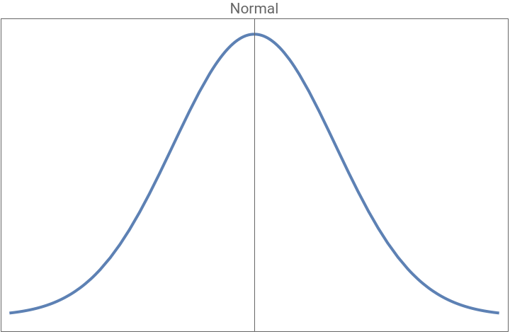
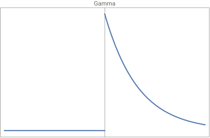
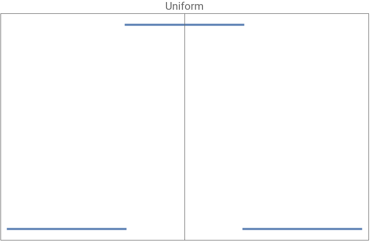
An important note: The graphs of these distributions were generated with a run of the distribution using “standard parameters”: in the case of a Normal distribution; μ = 0 and σ = 1, in the case of a Gamma distribution; α = 1 and β = 1, and in the case of a Uniform distribution; range = 1.
Initializing Weights from each Distribution
Initializing Weights from each Distribution
In[]:=
weightDistributions[distributionTypes_,params_]:=Module[{distribution,weightPlots,weights,distributions},distributions=MapThread[Switch[#1,"Normal",NormalDistribution[#2[[1]],#2[[2]]],"Uniform",UniformDistribution[{-#2[[1]],#2[[1]]}],"Gamma",GammaDistribution[#2[[1]],#2[[2]]],_,NormalDistribution[0,1]]&,{distributionTypes,params}];SeedRandom[1234];weights=Table[Flatten[Table[Module[{net=NetInitialize[NetChain[{3,LinearLayer[3],LinearLayer[3],LinearLayer[1]},"Input"->{3}],Method->{"Random","Weights"->distribution},RandomSeeding->Automatic]},Normal[NetExtract[net,{All,"Weights"}]]],15]],{distribution,distributions}];weightPlots=Table[Column[{Histogram[weights[[i]],PlotLabel->distributionTypes[[i]]<>" Distribution",Frame->True,ImageSize->{300,150}]}],{i,Length[distributionTypes]}];Column[{Style["Distributions of Weights by Initialization Distribution",Bold,14,TextAlignment->Center],Grid[{{Row[weightPlots,Spacer[10]]}},Alignment->Center]}]]
This function was created to provide a visual representation of weights initialized from each of the “main distributions” that this project will cover. It allows the user to enter a list of the distributions for which they wish to generate weights, followed by a list of parameters for each distribution. With these inputs, it runs the built-in NetInitialize function to randomly generate weights from each distribution-parameter pair.
Rasterize[weightDistributions[{"Normal","Gamma","Uniform"},{{0,1},{1,1},{1}}]]

This call to the function weightDistributions generates a histogram of weights initialized from a Normal distribution with μ = 0 and σ = 1, a Gamma distribution with
α = 1 and β = 1, and a Uniform distribution with range = 1. As we can see the histogram of weights resembles the distribution from which they were generated for the most part, with small deviations since we’re obviously not generating infinitely many weights.
α = 1 and β = 1, and a Uniform distribution with range = 1. As we can see the histogram of weights resembles the distribution from which they were generated for the most part, with small deviations since we’re obviously not generating infinitely many weights.
Guide to “Output Plots” in this Project
Guide to “Output Plots” in this Project
The vast majority of findings in this project will be represented in the form of “output plots.” They are a visualization that was inspired by Stephen Wolfram’s work in his article “Can AI Solve Science?” that was published in March 2024. Output plots, as will be referenced henceforth, are plots of the outputs of 15 runs of a neural network (with architecture and activation function specified in the plot) that has weights initialized from a specific distribution with specific parameters (this will also be clearly indicated in the description of the output plot). Each run will be represented by a line of different color and will show the output of the neural network for inputs ranging from -3 to 3, so the whole output plot will contain 15 different colored lines, where each line is generated by weights initialized from the same distribution. The point of having 15 runs of each initialization is to show general trends and ensure that the output shown isn’t due to a random fluctuation (for example, if the normal distribution graph above was left-skewed in one initialization). An example of an output plot is shown below.
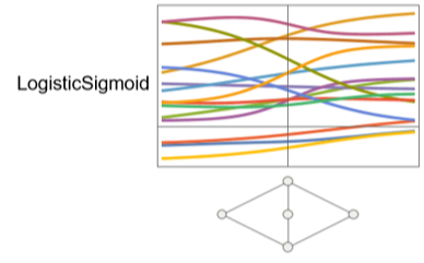
This output plot was generated from a neural network with the architecture shown below the plot (a single hidden layer) with the implementation of the LogisticSigmoid activation function and weights initialized from a normal distribution with μ = 0 and σ = 1.
Each line of outputs from -3 to 3 represents a run of this neural network (each of these runs will be slightly different because although the weights are initialized from the same exact distribution, they are still initialized randomly and will be distributed differently), and the plot as a whole shows a trend in the outputs that will be explained in future sections.
An important note is that these output plots will be generated in large grids to allow for easy comparisons between the output plots for different combinations of functions, distributions, and depths. These collections of plots take a long time to render, so the built-in Wolfram Language function Rasterize was used to convert each grid of plots into an image that is much less computationally intensive to render.
Linear Activation Functions
Linear Activation Functions
Most activation functions are either non-linear or piecewise, but it is possible to construct a neural network with only linear functions, and the results from this are essential to understand before moving on to more complex network structures.
Linear Regression
Linear Regression
When we create a neural network with each layer having a fully linear activation function (LinearLayer), each layer simply outputs a linear combination of the outputs of the previous layer. Mathematically, this shows itself as
Layer Output
where is a matrix of weights and is the value of the bias. It’s important to note that you could apply this operation infinite times and the output would still be a linear combination of the original weights and biases. The proof for this is outlined below.
(x+)+x++()x+(+) and is a matrix, and + is a vector, making this a linear transformation.
Because of this property of linear transformations, a neural network with solely linear activation functions, or in other words: only linear layers, becomes a linear regression model. This portion of the project will examine how changes in the distributions of weights and biases affect the outputs of a linear regression neural network and how the behavior changes with varying depths.
Layer Output
Wx+b
where
W
b
W
2
W
1
b
1
b
2
W
2
W
1
W
2
b
1
b
2
W
2
W
1
W
2
b
1
b
2
W
2
W
1
W
2
b
1
b
2
Because of this property of linear transformations, a neural network with solely linear activation functions, or in other words: only linear layers, becomes a linear regression model. This portion of the project will examine how changes in the distributions of weights and biases affect the outputs of a linear regression neural network and how the behavior changes with varying depths.
Creating Output Plots for Linear Regression Models
Creating Output Plots for Linear Regression Models
In[]:=
LinearRegressionNetworkPlot[depths_,distributionType_,params_]:=Module[{netInit,f,plots,depth,distribution,title},distribution=Switch[distributionType,"Normal",NormalDistribution[params[[1]],params[[2]]],"Uniform",UniformDistribution[{-params[[1]],params[[1]]}],"Gamma",GammaDistribution[params[[1]],params[[2]]],_,NormalDistribution[0,1]];SeedRandom[1234];title="Outputs of Linear Regression Network with Weights initialized from a "<>distributionType<>" distribution";plots=Table[With[{netInit=NetChain[Append[Catenate@Table[{3,LinearLayer[3]},depth],LinearLayer[1]],"Input"->{3}]},Column[{Plot[Evaluate@Flatten@Table[Module[{net=NetInitialize[netInit,Method->{"Random","Weights"->distribution},RandomSeeding->Automatic],f},f[x_?NumericQ]:=net[{x,x,x}];SetAttributes[f,Listable];f[x]],15],{x,-3,3},PlotRange->Full,Frame->True,FrameTicks->None],Style["depth = "<>ToString[depth],Italic,12,Gray]}]],{depth,depths}];Column[{Style[title,Bold,14],Row[Riffle[plots,Spacer[20]]]}]]
This function generates output plots that have weights generated from either Normal, Gamma, or Uniform distributions. Based on the distribution type, it takes either one or two parameters for generating the distribution (for a normal distribution this would be σ, for a gamma distribution it would be α and β, and for a uniform distribution it would be the range). It generates an output plot for each distribution type for different depths (also taken as an input in list form), showing a clear progression of the complexity of outputs as depth increases and providing visual warnings of gradient loss or explosion. Note that in this structure, each linear layer of the neural network takes in a 3-dimensional vector (used because this is the standard), and the final layer outputs a one-dimensional vector for the result of the entire neural network.
The Effect of Depth on Output Complexity
The Effect of Depth on Output Complexity
Rasterize[Column[{LinearRegressionNetworkPlot[Range[8],"Normal",{0,1}],LinearRegressionNetworkPlot[Range[8],"Gamma",{1,1}],LinearRegressionNetworkPlot[Range[8],"Uniform",{1}]}]]
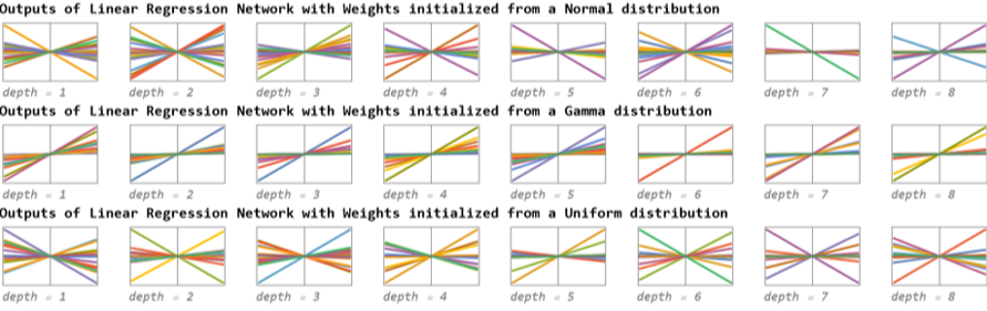
Plotting the output graphs for depths 1 through 10 (using a standard normal distribution for purposes of familiarity and ease of computation) shows almost no correlation between the depth of the network and the complexity of the outputs. In fact, running this with different random seeds produces very different output graphs, where different depths produce outputs of completely different shapes with no clear trend between said shapes. This is largely explained from the earlier referenced property of linear transformations where multiple linear transformations combine to create a single, slightly different linear transformation. This means that without a non-linear activation function, the network is unable to learn many of the patterns in training data and this greatly impedes the effectiveness of the model. In other words, any arbitrarily large neural network will only linear layers behaves like a neural network with just one linear layer.
Another interest aspect of the plots above comes in the difference between the shapes of the output graphs of the neural networks generated by a gamma distribution versus the output graphs of the neural networks generated by a normal or uniform distribution. This difference is caused by the definition of the distributions: while normal and uniform distributions can take upon negative values, a gamma distribution is restricted to producing strictly nonnegative values. This means that without negative weights, the neural network generated from a gamma distribution contains only positive or zero weights and produces negative outputs for negative input values and positive outputs for positive input values. In other words, the slope of all of the output graphs for gamma distribution are always positive.
Another interest aspect of the plots above comes in the difference between the shapes of the output graphs of the neural networks generated by a gamma distribution versus the output graphs of the neural networks generated by a normal or uniform distribution. This difference is caused by the definition of the distributions: while normal and uniform distributions can take upon negative values, a gamma distribution is restricted to producing strictly nonnegative values. This means that without negative weights, the neural network generated from a gamma distribution contains only positive or zero weights and produces negative outputs for negative input values and positive outputs for positive input values. In other words, the slope of all of the output graphs for gamma distribution are always positive.
Weight Distribution vs Output Distribution
Weight Distribution vs Output Distribution
In[]:=
weightDistributionOutputPlot[depth_,distributionType_,params_]:=Module[{distribution,weights,net,inputData,outputData},distribution=Switch[distributionType,"Normal",NormalDistribution[params[[1]],params[[2]]],"Uniform",UniformDistribution[{-params[[1]],params[[1]]}],"Gamma",GammaDistribution[params[[1]],params[[2]]],_,NormalDistribution[0,1]];SeedRandom[1234];net=NetInitialize[NetChain[Append[Catenate@Table[{3,LinearLayer[3]},depth],LinearLayer[1]],"Input"->{3}],Method->{"Random","Weights"->distribution},RandomSeeding->Automatic];weights=Flatten[Normal[NetExtract[net,{All,"Weights"}]]];inputData=Table[{x,0,0},{x,-3,3,0.1}];outputData=net[inputData];Column[{Histogram[weights,PlotLabel->distributionType<>" Distribution of Weights",Frame->True,ImageSize->{250,150}],ListPlot[Transpose[{Range[-3,3,0.1],Flatten[outputData]}],PlotLabel->"Network Output",Frame->True,ImageSize->{250,150},Joined->True]}]]
This function is similar to one previously defined, but in addition to generating a distribution of weights for a given distribution and parameters, it also plots the output for a network that contains exactly that distribution of weights for inputs from -3 to 3, intending to visually represent the effect weight distribution has on a linear regression neural network’s outputs. There is only one run of the neural network here, because there is no variation (the weights are set).
Rasterize[Row[Flatten[Table[Table[weightDistributionOutputPlot[2,distribution,Switch[distribution,"Normal",{0,1},"Uniform",{1},"Gamma",{1,1}]],3],{distribution,{"Normal","Uniform","Gamma"}}]]]]
Out[]=
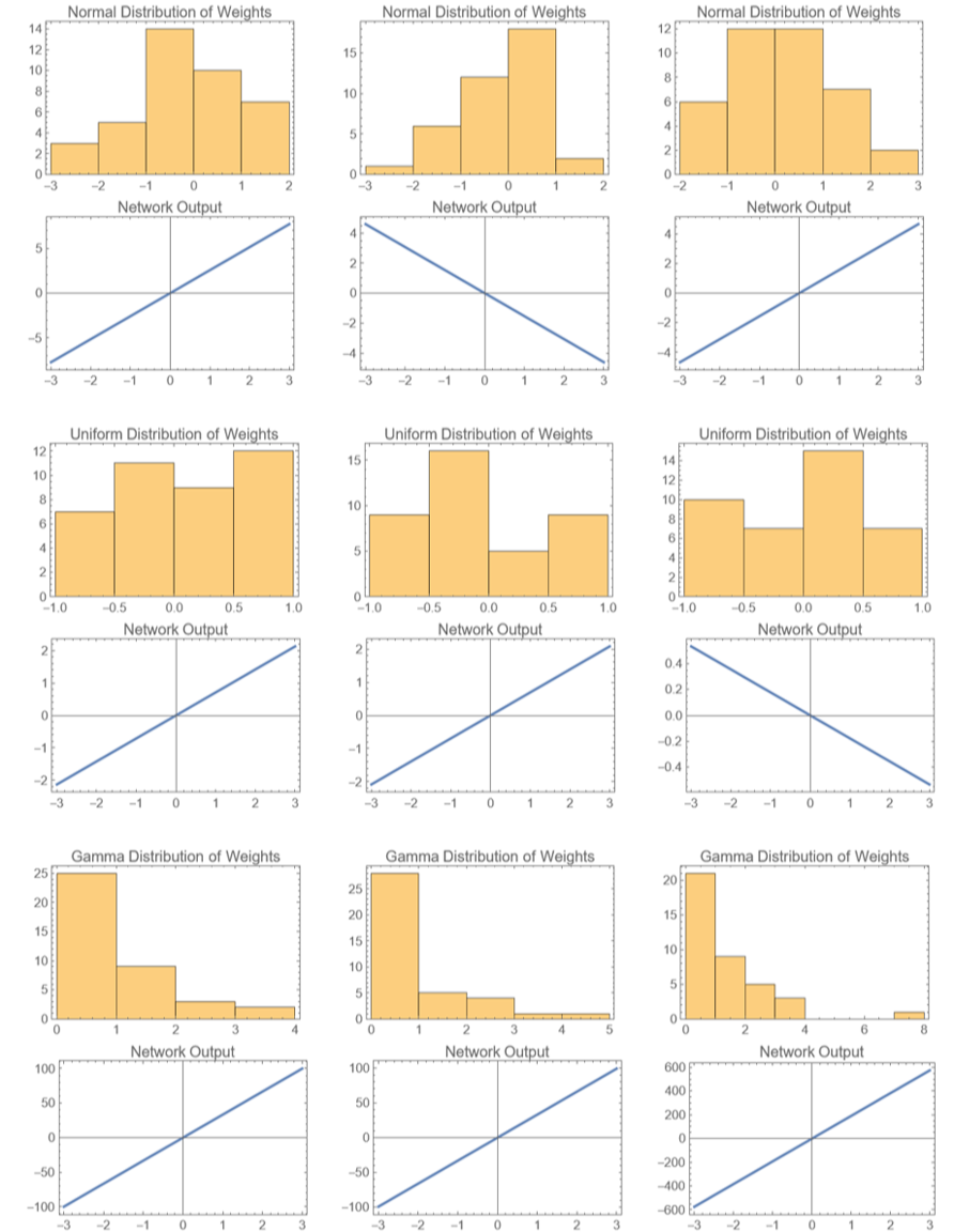
The graphs above are paired, with each Network Output being generated by a neural network initialized with the distribution of weights above it. At first glance, the correlation between the distributions and the outputs doesn’t seem to exist. Whether or not the mean of the weight distribution is above 0 would be the most obvious thing to check, but it doesn’t have an effect on the slope of the output. The slope almost feels random, but because the output plot is derived directly from linear combinations of the weights, this can’t be true. The relation becomes clear when considering the skew of the distributions of weights. Left-skewed weight distributions cause output plots with negative slopes, while right-skewed distributions cause a positive slope.
The explanation for this is again due to a property of linear transformations. If the majority of the entries of the weight matrix are negative, then multiplying the input by that matrix will result in a positive value when the input is negative and a negative value when the input is positive, leading to a negative slope in the output plot. If the majority of entries in the weight matrix are positive, then the resulting output will be negative for negative inputs and positive for positive inputs, resulting in a positive slope. A left-skewed graph means more negative weights, and a r0ght-skewed graph means more positive weights.
The explanation for this is again due to a property of linear transformations. If the majority of the entries of the weight matrix are negative, then multiplying the input by that matrix will result in a positive value when the input is negative and a negative value when the input is positive, leading to a negative slope in the output plot. If the majority of entries in the weight matrix are positive, then the resulting output will be negative for negative inputs and positive for positive inputs, resulting in a positive slope. A left-skewed graph means more negative weights, and a r0ght-skewed graph means more positive weights.
One Non-Linear Activation Function
One Non-Linear Activation Function
The addition of a non-linear activation function to a neural network composed of linear layers renders the earlier property about linear transformations combining to create other linear transformations irrelevant. Because these activation functions are non-linear, iterating them upon each other results in much more complex relations than simply another version of the activation function. This allows these types of models to understand and replicate more complex relationships within training data and allows the model to attain a much higher level of fitting.
This portion of the project will examine how changes in the distribution of weights and the depth of the neural network affect the output of a given neural network with the implementation of a single activation function in a hidden layer. While this may seem almost identical to the previous portion, there are key differences when non-linear functions are introduced (namely the depth will actually play a role in the complexity of the output graphs). Additionally, because of this new affecting variable, we have to consider the phenomena that are gradient loss and gradient explosion. Gradient loss occurs when gradient get pushed toward 0 as they’re passed through the hidden layers of the neural network, and this is a problem because that mean the neural network is unable to learn, leading to long training times, stagnation in the performance of the neural network as a whole, and under-fitting.
Gradient explosion, on the other hand, is almost the exact opposite; gradients grow out of control as they’re passed through the hidden layers, and by the time they reach the last layer, they can become so large that they update the weights too drastically and cause oscillations during training. Like gradient loss, gradient explosion can result in long training times, but it leads more often to overfitting. Further sections of this portion of the project will define functions to help identify when gradient loss or gradient explosion are occurring and how to initialize the neural network in a manner that alleviates the issues.
Activation Functions
Activation Functions
While there are countless activation functions that can be implemented within a neural network, this project will make use of five of the most popular, selected because they provide an opportunity to compare the effects of different characteristics of activation function (e.g. fully non-linear vs piecewise linear, limited range of output vs non-limited range of output, periodic vs aperiodic, etc). These functions have been outlined in a grid below.
Testing Parameters for Normal Distributions
Testing Parameters for Normal Distributions
We’ll start with generating weights from a basic Normal distribution. With this distribution, we’ll be examining the effect of changing the standard deviation and network depth on the complexity of graphs of outputs.
This function takes in parameters for a list of activation functions, a list of depths, and a standard deviation. It uses these parameters to generate a grid that consists of output plots for each activation function paired with each depth, initializing weights from a normal distribution with the inputted standard deviation. Why is this useful? The behavior of the untrained neural network is what will dictate the speed and stability of the training process. In this case, we want to avoid extremes, as overly “messy” graphs can result in gradient explosion and a very unstable training process, while very flat graphs can result in gradient loss and a halt in training.
From the graphs of the outputs, we can see a result that, for the most part, seems to have been obvious. The non-linear functions Sin and Tanh retain a fairly high frequency in their graphs, and this frequency only increases as the depth increases. From this we can tell that perhaps having too many layers with non-linear activation functions isn’t a good idea as it could quickly lead to model instability. On the other hand, the piecewise functions Ramp and Threshold exhibit almost the exact opposite behavior. Starting out almost as complicated as Sin and Tanh, they quickly dwindle in frequency as the network depth increases, and this can be attributed to the fact that for Threshold, as more layers are added, the outputs become either 0 or 1, and there is little variation in outputs for different inputs. For Ramp, we see that the graphs don’t ever lose all of their character, instead seemingly reaching a kind of “asymptote of flatness”, in which the graphs remain a bit too smooth for robust training but workable. The real outlier here is Logistic Sigmoid. Why does a non-linear function reach full flatness before either of the linear activation functions? Sigmoid is limited to producing outputs between 0 and 1, and a cursory glance at the function’s graph shows us that it’s first derivative rapidly approaches 0 at extreme values, whether those be positive or negative. Repeatedly applying this function over multiple layers pushes outputs toward these extrema and results in a complete loss of gradient that stops training entirely, highlighting a problem with the Logistic Sigmoid activation function (one that can be tackled with specialized initializations that will be covered later in this project).
Optimal Standard Deviation for Varying Network Depths and Activation Functions
Optimal Standard Deviation for Varying Network Depths and Activation Functions
The output plots above showed a problem with initialization for certain activation functions. To limit the scope of this problem, this project will explore functions to optimize the standard deviation. What is the “optimal” standard deviation? In this case, it’s the standard deviation, σ, that creates a normal distribution with mean μ and standard deviation σ that initializes weights such that depth before gradient loss or gradient explosion occurs is maximized, leading to stable training.
Nothing special here; we’re just initializing a Neural Network with parameters for the activation function, network depth, and standard deviation of the distribution of weights.
This is the function used to evaluate outputs of the neural network (important because we’re trying to measure and plot the “smoothness” of the outputs.
This functions takes in inputs for activation function and depth and runs normalInitializeNet with a neural net of that structure for each of the standard deviations in the list stdDevs, with 15 runs per initialization (to have a large enough sample size). With these outputs it runs normalEvaluateNet from -3 to 3 with a step size of 0.01 (in order to try to emulate a continuous variable), and then measures the variance of the list of outputs. This measure is important, because the variance is an almost direct indicator of whether the neural network will devolve into either gradient loss or explosion.
This normalPlotVariance function plots the mean variances against the standard deviations for a certain activation function and depth. In addition to providing a visual representation of the normalOptimalStdDev function, it shows the trend in mean variance with increasing standard deviation and clearly indicates the optimal standard deviations for either minimizing or maximizing the variance.
These two side-by-side graphs represent the plots of variance measure for neural networks composed of weights initialized from normal distributions with varying standard deviations. The obvious difference comes in which activation functions were used, with the first graph representing LogisticSigmoid and the second representing Sin. The goals when creating a network architecture with these two functions are completely different: with LogisticSigmoid, it’s important to maximize the variance measure so that we can prevent vanishing gradients, and with Sin, minimizing the variance measure ensures prevention of gradient explosion. The plots show us that increasing standard deviation corresponds to increasing variance measures, and indicates that for a LogisticSigmoid activation, we want as high a standard deviation as possible, while for a Sin activation, we want a standard deviation somewhere between 1 and 4. An important note comes with the scaling of the ranges of each graph (one is on a scale to 70, while the other has values ranging up to 175).
Gamma Distributions
Gamma Distributions
The main changes from generating weights with a normal distribution to generating weights with a gamma distribution are that the weights will always be nonnegative in the latter case and that there are now two metrics to examine: α and β instead of just σ.
This gammaNetworkPlot function works very similarly to the normalNetworkPlot function, with the key difference coming in the fact that it takes parameters for α and β instead of σ.
The functions above are the same as the ones for Normal distribution, just tailored to the parameters of a Gamma distribution.
Plotting a 3-dimensional graph to visually represent the effect of changing α and β on the variance measure. The point is both to discover the optimal combination and to be able to visualize the derivative of variance measure at certain points on the graph.
These two 3D visualizations aren’t that different from the two that were developed to find the optimal standard deviation (other than the obvious difference: in this case optimization of two variables is required). Both visualizations above represent the variance measures for neural networks with weights initialized from a Gamma distribution with the difference coming in that the visualization on the left has a networks that was constructed with a LogisticSigmoid function, while the one on the right represents a network that was constructed with a Sin function. Testing values of α and β from 1 to 10 with a step size of 1 (interpolating to create a continuous graph) shows the general ranges of α and β that optimize the Gamma distribution for each activation function.
As always, with LogisticSigmoid, the higher the variance measure the better, so as shown in the graph, best practice would be to minimize α and maximize β. Since the range of the variance measures on the z-axis only range up to 20, gradient explosion is never a worry. On the other hand, with Sin, the range of the variance measures goes up to 500, and variances that high make gradient explosion almost inevitable. Because of this, the optimal combinations of α and β occur along the part of the graph where the variance measure starts to change from a flat sheet at almost zero to an increasing exponential function.
As always, with LogisticSigmoid, the higher the variance measure the better, so as shown in the graph, best practice would be to minimize α and maximize β. Since the range of the variance measures on the z-axis only range up to 20, gradient explosion is never a worry. On the other hand, with Sin, the range of the variance measures goes up to 500, and variances that high make gradient explosion almost inevitable. Because of this, the optimal combinations of α and β occur along the part of the graph where the variance measure starts to change from a flat sheet at almost zero to an increasing exponential function.
Uniform Distribution
Uniform Distribution
Now, the main defining characteristic of weights generated from this distribution is that they will usually be more spread out than those from a normal distribution, or in other words, they will exhibit a higher standard deviation.
This uniformNetworkPlot function works exactly like the normalnetworkPlot function, except instead of σ, it takes in a range parameter that defines a uniform distribution from -range to range.
Finding Optimal Range to prevent Gradient Loss/Gradient Explosion
Finding Optimal Range to prevent Gradient Loss/Gradient Explosion
Identical to the functions for Normal and Gamma distribution with the exception of the substitution of range for σ, or α and β.
Testing different ranges to plot the effect of wider selections of weights and more extreme values on the outputs for certain functions.
Function to plot the mean variance against the range and find correlations between the two variables.
These plots are in the exact same format as the ones for weights initialized from a normal distribution, but obviously the independent variable in this case is range instead of σ. The difference is that the values for variance are much lower. LogisticSigmoid only reaches 25, while Sin only reaches 80 as opposed to the values of 70 and 200 that a normal distribution produced. Why is this the case?
The uniform distribution is equally likely to generate any of the values in its range, and while this lends itself to a higher variance, that variance is in the distribution of weights not the outputs. With a higher distribution in the weights, this makes it more likely that the weights will have cancelling effects on each other, then resulting in outputs with a lower variance. Again, we see that a high range is important with LogisticSigmoid, but since even the highest range on this graph results in an obscenely low variance, it seems safe to conclude that generating weights from a uniform distribution doesn’t pair well with using LogisticSigmoid as an activation function. On the other hand, this distribution works almost perfectly with Sin (almost all the y-values in this graph are in the perfect range between 30 and 60 that lends itself to a stable training process).
The uniform distribution is equally likely to generate any of the values in its range, and while this lends itself to a higher variance, that variance is in the distribution of weights not the outputs. With a higher distribution in the weights, this makes it more likely that the weights will have cancelling effects on each other, then resulting in outputs with a lower variance. Again, we see that a high range is important with LogisticSigmoid, but since even the highest range on this graph results in an obscenely low variance, it seems safe to conclude that generating weights from a uniform distribution doesn’t pair well with using LogisticSigmoid as an activation function. On the other hand, this distribution works almost perfectly with Sin (almost all the y-values in this graph are in the perfect range between 30 and 60 that lends itself to a stable training process).
Special Initializations
Special Initializations
Because there are some issues when generating weights from the standard distributions for some activation functions (namely those that resemble Logistic Sigmoid), researchers have come up with a couple of special initializations to enhance the training process when using those functions. This section will generate similar plots for these initializations in a bid to determine whether there are some parameters that when inputted into a Normal, Gamma, or Uniform distribution will perform better than the special initializations.
Xavier Initialization
Xavier Initialization
This function creates a grid of output plots for combinations of the activation functions and depths inputted into the function, and generates weights from a normal distribution with standard deviation in accordance with the Xavier initialization.
So, as we can see, the Xavier initialization nicely tampered down the frequency of the Sin graph, but didn’t seem to do much to improve the gradient loss problem that LogisticSigmoid has been straddled with. In fact, as soon as the depth increases past 1, the output plots are almost flat. Tanh and Ramp fare slightly better, not being completely flat in any of the frames shown in this grid of output plots, but Threshold falls into vanishing gradients shortly after LogisticSigmoid. This reveals that LogisticSigmoid doesn’t work well on it’s own, often leading to untrainable neural networks. However, as later sections of this project show, it performs far better when combined with other activation functions.
If having a neural network with only LogisticSigmoid is absolutely necessary, there’s still an important conclusion to be drawn from this. Checking back to the plots from the Gamma distribution shows that minimizing α and maximizing β for a Gamma distribution will produce better results than this specialized initialization.
If having a neural network with only LogisticSigmoid is absolutely necessary, there’s still an important conclusion to be drawn from this. Checking back to the plots from the Gamma distribution shows that minimizing α and maximizing β for a Gamma distribution will produce better results than this specialized initialization.
He Initialization
He Initialization
This function works identically to the Xavier initialization function (obviously with the formula for standard deviation being altered to fit with the He initialization instead).
As the He (Kaiming) initialization was defined specifically for the Ramp activation function, we’ll examine its effects on the output plots for that activation function first. As the depth increases, the output plots begin to flatline, and while it doesn’t occur as rapidly as it did with a non-specialized normal distribution or uniform distribution, it still occurs. Again, we find that there’s a more suitable alternative to this initialization that works better with the Ramp function. Revisiting the output plots for the Gamma distribution shows that for Ramp, vanishing gradients never occurred, no matter what depth the network reached.
As for the other activation functions, the He initialization performs almost identically to the non-specialized normal and uniform distributions, making it clear that this initialization holds little value for neural networks with only one activation function. This is true for most specialized initializations: the vast majority of practical usages of neural networks come with complex architectures with multiple activation functions, so specialized initializations have been developed with these architectures in mind, not simple single function networks.
As for the other activation functions, the He initialization performs almost identically to the non-specialized normal and uniform distributions, making it clear that this initialization holds little value for neural networks with only one activation function. This is true for most specialized initializations: the vast majority of practical usages of neural networks come with complex architectures with multiple activation functions, so specialized initializations have been developed with these architectures in mind, not simple single function networks.
Combining Activation Functions to Create More Complex Neural Networks
Combining Activation Functions to Create More Complex Neural Networks
So far, this project has focused on only the simplest of neural network architectures with a linear regression model and single activation function models, as these provided the clearest representations of the effect of different distributions of weights on the training process. However, this upcoming section will focus on more complex neural network architectures with multiple hidden layers of different activation functions. We’ll discover how well the previously outlined relationships hold for these more complex models and will outline new correlations that work for these architectures and which combinations of activation functions perform best.
Two Activation Functions
Two Activation Functions
This neural network architecture starts with an input layer, followed by consecutive hidden layers of each activation function, finally ending with an output layer. For example, if the two activation functions were Ramp and LogisticSigmoid, the structure would be input, Ramp, LogisticSigmoid, output. This applies only for a depth 1 network, though. The depth represents the amount of times the hidden layer combination is repeated. So, for depth 2, it would be input, Ramp, LogisticSigmoid, Ramp, LogisticSigmoid, output, and for depth 3 it would be input, Ramp, LogisticSigmoid, Ramp, LogisticSigmoid, Ramp, LogisticSigmoid, output.
Normal Distribution
Normal Distribution
The most obvious thing about this grid of outputs is that when the depth is odd, the graphs are flat, while when the depths are even, they become incredibly complex. It’s logical that for depth 1 the graphs start out relatively flat, but why are the graphs for depth 3 so flat? At first, it seemed to be a result of random chance, but multiple runs of this function produced similar results, and the most plausible explanation seems to be that the third layer of functions partially smooths out the variations introduced by the second layer, and then the fourth layer reintroduces variations into the output plots. As for why the depth 4 graphs are so much more complex than those for depth 2, it’s because there’s much more room for variation with the extra 2 layers.
The other important observation to make is that there is no readily noticeable difference between the output plots for each combination of functions. Why do Ramp and LogisticSigmoid produce the same type of graphs as Tanh and Sin? There are two main factors that contribute to this: firstly, because these output plots are generated from untrained neural networks with randomly initialized weights, the network hasn’t been able to fit itself to each activation function, so the results don’t vary too much by function combination. Secondly, these activation functions have a lot in common (for example, both Sin and LogisticSigmoid are bounded from 0 to 1), and the small differences that are created by varying them are far outshone by the differences when modifying the depth of the neural network.
The other important observation to make is that there is no readily noticeable difference between the output plots for each combination of functions. Why do Ramp and LogisticSigmoid produce the same type of graphs as Tanh and Sin? There are two main factors that contribute to this: firstly, because these output plots are generated from untrained neural networks with randomly initialized weights, the network hasn’t been able to fit itself to each activation function, so the results don’t vary too much by function combination. Secondly, these activation functions have a lot in common (for example, both Sin and LogisticSigmoid are bounded from 0 to 1), and the small differences that are created by varying them are far outshone by the differences when modifying the depth of the neural network.
Gamma Distribution
Gamma Distribution
This function accomplishes the same purpose as the normalTwoFunctionNetworkPlot function, except instead of initializing weights from a normal distribution, it initializes from a gamma distribution with
α and β both set to 1.
α and β both set to 1.
Now, the obvious fact is that the grid of output plots for the gamma distribution is the almost perfect opposite of the output plots of the normal distribution. Instead of having the even depths have increased complexity, in this case, depths 1 and 3 are the ones that have high frequencies. The most plausible explanation for this is similar to the one provided for normal distributions: depth 1 has fairly high complexity because the combination of two activation functions when there are no negative weights returns non-linear outputs. Then, depth 2 plays the role that depth 3 formerly took, smoothing out the outputs from the first two hidden layers, when depth 3 reintroduces them (creating even higher complexity because of the increased potential for non-linear combinations).
Another, less obvious, observation can be made when examining specifically the output plots for depth 1 and 3. For depth 1, the complexity in output graphs comes only for negative inputs, while for depth 3, it comes for only positive outputs. Why is only half the graph complex, and why does the half change by depth? This is a question that will likely need further examination, but the best explanation that can be offered from these results is that when each function is applied only once, small changes in the distribution of weights greatly affect the outputs for negative inputs, while when each function is applied three times, small changes only affect the outputs for positive inputs. Again, this isn’t a completely satisfactory explanation, and this is an area where future research will be required to explain these results.
Another, less obvious, observation can be made when examining specifically the output plots for depth 1 and 3. For depth 1, the complexity in output graphs comes only for negative inputs, while for depth 3, it comes for only positive outputs. Why is only half the graph complex, and why does the half change by depth? This is a question that will likely need further examination, but the best explanation that can be offered from these results is that when each function is applied only once, small changes in the distribution of weights greatly affect the outputs for negative inputs, while when each function is applied three times, small changes only affect the outputs for positive inputs. Again, this isn’t a completely satisfactory explanation, and this is an area where future research will be required to explain these results.
Uniform Distribution
Uniform Distribution
This function accomplishes the same purpose as the two above, with the parameters being tailored toward a uniform distribution.
In this case, the uniform distribution is the outlier: here, it seems that neither the depth nor the combination of activation functions matters. This wasn’t particularly a problem for single activation functions, but having an almost equally distributed amount of positive and negative weights with two activation functions greatly increases the likelihood that the different layers with counteract each other’s effects and end up producing flat-lining outputs. This result provides an explanation for the reason that Uniform distributions are rarely used to initialize neural networks: almost all practical use neural networks use a combination of two or more activation functions with multiple hidden layers, and initializing weights from a uniform distribution would hugely impede the speed of the training process.
Multiple Activation Functions
Multiple Activation Functions
This architecture is fairly similar to the one outlined for two activation functions, with the obvious difference being that there is three or more activation functions before they begin to be repeated. So, for example if we had three functions to use: (Sin, Tanh, and Threshold), then for depth 1 the architecture would be input, Sin, Tanh, Threshold, output, and for depth 2 it would be input, Sin, Tanh, Threshold, Sin, Tanh, Threshold, output.
Normal Distribution
Normal Distribution
Now, we see that as we subsequently apply more and more activation functions, the outputs seem to become more and more flat. Here, it’s not terrible for some combinations (namely Tanh, Sin, and Ramp) and (Tanh, Sin, and LogisticSigmoid), but why are these so much more flat than those for combinations of two activation functions? The best explanation this project can offer is that many of the activation functions used here produce outputs with low variation when taking inputs close to 0, and because we are initializing from an normal distribution, this causes graphs with low variation. This isn’t a perfect explanation, though, and some of the behaviors of these output plots remains incomprehensible, so longer iterations than are supported by this project (for example, trying every possible order of activation functions and seeing the results, or modeling the change in weights between layers) is something that will be needed. The latter is a planned extension of this project and will hopefully uncover more.
Gamma Distribution
Gamma Distribution
This function is the same as the above, but specifically made to take parameters for a Gamma distribution
Since, α was set to 1 before generating this grid of plots, it means the weights are being initialized from an exponential (logarithmic) distribution where all of the values are positive. This grid has more life than the one that was generated from a normal distribution and actually allows for distinctions to be made on which activation functions work best together. Sin, Ramp, and Logistic Sigmoid create completely flat graphs, while combinations of Tanh, Sin, and Ramp along with Tanh, Ramp, and Logistic sigmoid provide ample variation that might allow for a decently stable training process. To examine better which orders are best for which distribution the results of each possible ordered combination would have to be checked, and this would have to be iterated over standard deviations and depths. However, this does show an increasingly obvious trend from this project of the Gamma distribution outperforming the Normal distribution (this will be expanded upon later).
Uniform Distribution
Uniform Distribution
Function for output plot with multiple activation functions with a Uniform distribution.
As expected, the Uniform distribution again produces the flattest graphs out of the three for complex structures. The explanation for this is the same as for two activation functions: having weights equally distributed about zero increases the probability that different activation functions nullify each other’s effects and end up producing linear outputs. Here, it’s hard to imagine a successful training process, especially with Sin, Ramp, and Logistic Sigmoid, where learning might cease at the first depth. It likely wouldn’t change the results but testing with larger ranges might provide some insight on making a Uniform distribution viable.
Conclusion
Conclusion
The purpose of this project was to explore the effects of different initializations of weights on the outputs of untrained neural networks, and as we’ve now covered different depths, architectures, and activation functions, there is enough of a result to outline some conclusions about these effects (as this is only an exploratory project with limited resources and time limit, not all possible permutations have been tested, so there is still some uncertainty about these conclusions that will be covered alongside each one).
After testing the 3 main distribution types (Normal, Gamma, and Uniform) over different depths and combinations of activation functions, it was clear that the Gamma distribution far outperformed expectations, producing outputs that indicated that it’s neural networks were at least as suitable for training as those that had weights initialized from a Normal distribution. When optimized for the α and β values that prevented gradient loss or explosion, the Gamma distribution even outperformed the Xavier and He initializations for neural networks with a singular activation function (this wasn’t tested for more complex architectures, so no definitive assessments can be made with regards to those, however, this result on its own is quite surprising). All of these results indicate that the Gamma distribution has more potential for weight and bias initialization in neural networks than is currently being utilized.
While the Gamma distribution had the most favorable performance, the Normal and Uniform distributions also provided impressive results when they were initialized with certain σ and range. The importance of these parameters was very surprising: just a small shift can completely change the shape of the output plot and be the difference between a smooth training process or a vanishing gradient problem. As this was extrapolated to more complex architectures and combinations of activation functions, these differences became harder to track and seemingly even more arbitrary, showing that neural networks (especially the ones that are put into practical use) are incredibly dependent upon the minute relations between their weights.
Implications for Future Research
Implications for Future Research
While the relations outlined above are undoubtedly important and fascinating, there were some limitations on this project (namely the time limit) that prevented exhaustive testing of certain combinations. A natural continuation of this project would be to generate output plots for all possible combinations of activation functions at higher depths and more complex architectures to paint a better understanding of why the output plots behave in this manner.
The other natural avenue that would likely yield results helping in the real world would be to determine how well the output plots predict post-training performance of the neural network and to see if the initialization of weights have any importance past reducing the computational intensity and runtime of the training process. If this analysis showed that there was some implications for post-training performance, then modeling the behavior of untrained neural networks and choosing the correct initialization would likely attract far more than the cursory research that has been done in this field.
The other natural avenue that would likely yield results helping in the real world would be to determine how well the output plots predict post-training performance of the neural network and to see if the initialization of weights have any importance past reducing the computational intensity and runtime of the training process. If this analysis showed that there was some implications for post-training performance, then modeling the behavior of untrained neural networks and choosing the correct initialization would likely attract far more than the cursory research that has been done in this field.
Acknowledgements
Acknowledgements
I would like to thank my mentor, Jack Heseltine, along with the Wolfram TAs for reviewing my work and suggesting improvements at every turn, without which this project certainly wouldn’t have turned out this satisfactorily. I would also like to thank Stephen Wolfram and all of the directors at the Wolfram Summer Research Program for providing the opportunity to conduct this research and learn Wolfram Language.
Bibliography
Bibliography
◼
Wolfram, S. (2024, March 27). Can AI solve science? Writings of Stephen Wolfram. https://writings.stephenwolfram.com/2024/03/can-ai-solve-science/
◼
Datta, L. (2020). A survey on activation functions and their relation with Xavier and He normal initialization. arXiv. https://arxiv.org/abs/2004.06632
◼
Skorski, M., Temperoni, A. & Theobald, M.. (2021). Revisiting Weight Initialization of Deep Neural Networks. Proceedings of The 13th Asian Conference on Machine Learning</i>, in <i>Proceedings of Machine Learning Research 157:1192-1207 Available from https://proceedings.mlr.press/v157/skorski21a.html.
CITE THIS NOTEBOOK
CITE THIS NOTEBOOK
Effects of randomly generated weights on outputs of untrained neural networks
by Sandeep Sethuraman
Wolfram Community, STAFF PICKS, July 11, 2024
https://community.wolfram.com/groups/-/m/t/3212548
by Sandeep Sethuraman
Wolfram Community, STAFF PICKS, July 11, 2024
https://community.wolfram.com/groups/-/m/t/3212548