After years of finding mathematics easy,
I finally reached integral calculus
and came up against a barrier.
Isaac Asimov
I finally reached integral calculus
and came up against a barrier.
Isaac Asimov
Reading the German Wikipedia entry on integration https://de.wikipedia.org/wiki/Integralrechnung
I saw that they mention a hard integral to solve:
I saw that they mention a hard integral to solve:
Out[]=
(1)
Which isn’t solved in this notebook (it’s in part 2), but a somewhat similar integral, which is explained in detail here:
https://www.youtube.com/watch?v=yKAoX4Ik0Q4
and also here:
https://math.stackexchange.com/questions/2174693/int-0-infty-frac1xe-ln2x-4-pi2-dx-keyhole-contour-o?rq=1
https://www.youtube.com/watch?v=yKAoX4Ik0Q4
and also here:
https://math.stackexchange.com/questions/2174693/int-0-infty-frac1xe-ln2x-4-pi2-dx-keyhole-contour-o?rq=1
The purpose of this notebook is to solve step by step the following integral and therefore proving its statement (and getting some nice corollaries in the appendix):
Out[]=
(2)
The area looks like this:
Out[]=
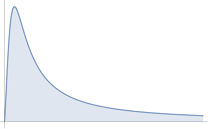
By now Mathematica up to 13.3 can’t solve this using Integrate. So this must really be a hard integral to solve:
In[]:=
Integrate,{x,0,∞}
x
(+)(+)
2
x
2
Log[x]
2
π
Out[]=
∞
∫
0
x
(+)(+)
2
x
2
π
2
Log[x]
But we can check it numerically:
In[]:=
NIntegrate,{x,0,∞}
x
(+)(+)
2
x
2
Log[x]
2
π
Out[]=
0.452941
Compare with the proposed solution:
In[]:=
N+
1
1+
2
1+
2
π
Out[]=
0.452941
And of course this is not a proof. On the other hand there is no reasonable doubt that it isn’t true. The first integral can’t even be checked numerically, which makes it even more fascinating.
First we have to know (or remember) the following about the logarithm in the complex plane:
Branch points fall into three broad categories: algebraic branch points, transcendental branch points, and logarithmic branch points.
The typical example of a branch cut is the complex logarithm. If a complex number is represented in polar form , then the logarithm of is
z=r
ϑ
z
Out[]=
However, there is an obvious ambiguity in defining the angle : adding to any integer multiple of will yield another possible angle. A branch of the logarithm is a continuous function giving a logarithm of for all in a connected open set in the complex plane. In particular, a branch of the logarithm exists in the complement of any ray from the origin to infinity: a branch cut. A common choice of branch cut is the negative real axis, although the choice is largely a matter of convenience.
ϑ
ϑ
2π
L(z)
z
z
The logarithm has a jump discontinuity of when crossing the branch cut. The logarithm can be made continuous by gluing together countably many copies, called sheets, of the complex plane along the branch cut. On each sheet, the value of the log differs from its principal value by a multiple of . These surfaces are glued to each other along the branch cut in the unique way to make the logarithm continuous. Each time the variable goes around the origin, the logarithm moves to a different branch.
2π
2π
Secondly we use this nice decomposition:
Out[]=
On the negative real axis (the branch cut discontinuity of log) we can write with the direction for the limit and , .
For example:
+
x∈
+
log(-x)=log(x)-π
For example
x=-3
In[]:=
Limit[Log[z],z->-3,Direction->]
Out[]=
-π+Log[3]
On the negative real axis we can write with the direction for the limit.
, , for example :
-
x∈
+
log(-x)=log(x)+π
x=-3
In[]:=
Limit[Log[z],z->-3,Direction->-]
Out[]=
π+Log[3]
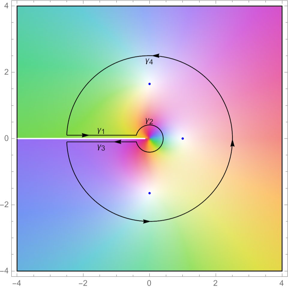
The integration path over the closed curve is marked with , , and . The value of the integral along this path is the sum of the residues inside.
And notice: The integration path does not cross the branch cut discontinuity on the negative real axis. And it doesn’t go through a singularity either. We are lucky, there is no singularity on the negative real axis.
γ
1
γ
2
γ
3
γ
4
And notice: The integration path does not cross the branch cut discontinuity on the negative real axis. And it doesn’t go through a singularity either. We are lucky, there is no singularity on the negative real axis.
Out[]=
γ
2
γ
4
γ
1
γ
3
Out[]=
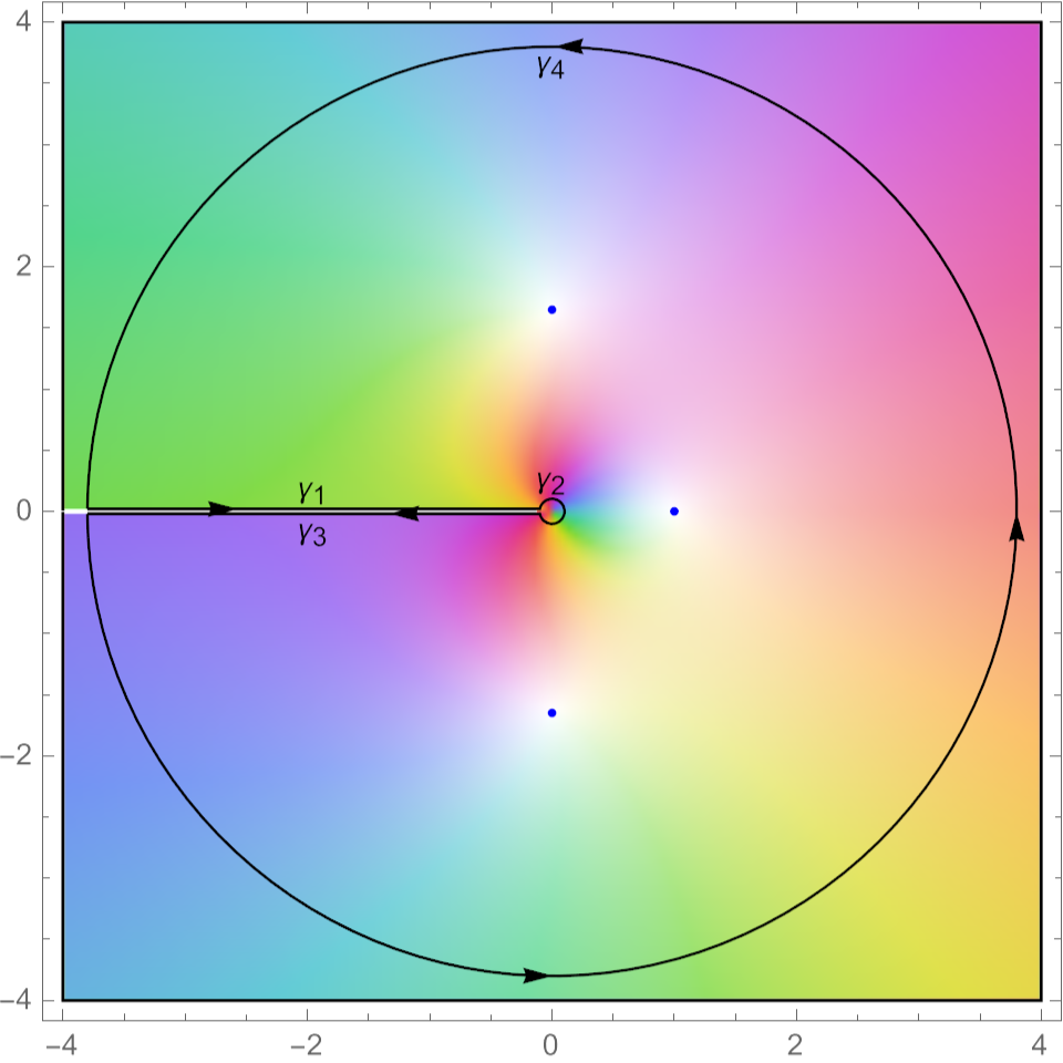
So we have f(z)z+f(z)z+f(z)z+f(z)z=2π∑Resf(z).In the above limit f(z)z and f(z)z go both to zero.
∫
γ
1
∫
γ
2
∫
γ
3
∫
γ
4
∫
γ
2
∫
γ
4
On the negative real axis (limit from ) this holds: f(z)z=x
+
∫
γ
1
0
∫
-∞
x
(+)(Logx+π)
2
x
Here the variables are changed by substitution and the integration boundaries are flipped:
IntegrateChangeVariables has problems with it!
IntegrateChangeVariables has problems with it!
Out[]=
On the negative real axis (limit from ) this holds: f(z)z=x
-
∫
γ
2
-∞
∫
0
x
(+)(Logx+π)
2
x
Another simple substitution:
IntegrateChangeVariables has problems with it!
IntegrateChangeVariables has problems with it!
Out[]=
So we have:+=-x
∫
γ
1
∫
γ
3
∞
∫
0
x
(+)(logz-π)
2
x
x
(+)(logz+π)
2
x
=2πx=2π∑Res
∞
∫
0
x
(+)+
2
x
2
log(x)
2
π
Out[]=
The residues are not zero at and the sum is:
1,±
In[]:=
ComplexExpandPlus@@MapResidue,{z,#}&,1,
z
(+)Log[z]
2
z
,-
Out[]=
1
1+
2
1+
2
π
Putting all together gives ( cancels on both sides):
2π
Out[]=
Q.E.D.
Appendix
Appendix
With “GlobalAbs” the poles (where the non vanishing residues may be) can be made better visible:
Using the same method one immediately gets these:
and so on …
case (5):
CITE THIS NOTEBOOK
CITE THIS NOTEBOOK
A hard integral to solve part one
by Oliver Seipel
Wolfram Community, STAFF PICKS, October 16, 2023
https://community.wolfram.com/groups/-/m/t/3050707
by Oliver Seipel
Wolfram Community, STAFF PICKS, October 16, 2023
https://community.wolfram.com/groups/-/m/t/3050707