Terminal Fall Velocity of a Single Spherical Particle in a Newtonian Fluid
Authors: Housam Binous and Ahmed Bellagi
Terminal Fall Velocity of a Single Spherical Particle in a Newtonian Fluid
Authors: Housam Binous and Ahmed Bellagi
Authors: Housam Binous and Ahmed Bellagi
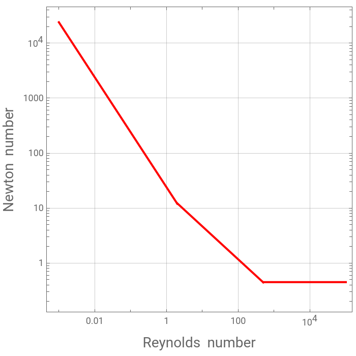
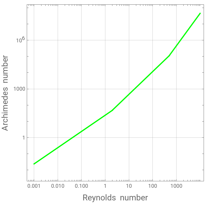
Newton number (also called the drag coefficient) and Archimedes number are plotted versus the Reynolds number for the laminar, transition and turbulent flow types using a log - log scale . Expressions and numerical examples of the terminal fall velocity of a single spherical particle in a Newtonian Fluid, for the three flow types, are given in this post . For laminar flow, the terminal velocity expression is given by the well - known Stokes' law . Measurement of terminal fall velocity has important applications such as viscosity determination (e . g . falling-ball viscometer) as well as decanter sizing .
Correlation between the Newton Number (also called the Drag coefficient) and the Reynolds number. Expression depends on flow type (i.e. laminar, transition, turbulent)
In[]:=
N
e
Plotting the Newton Number or the Drag coefficient versus the Reynolds number. We use log-log scale.
In[]:=
plt1=LogLogPlot[[x],{x,10^-3,10^5},PlotRangeAll,PlotPoints10000,GridLinesAutomatic,PlotStyle{Thick,RGBColor[1,0,0]},FrameTrue,ImageSize->350{1,1},AspectRatio->1,FrameLabel->{Style["Reynolds number",14],Style["Newton number",14]}]
N
e
Out[]=
Plotting the Archimedes Number (Ar= Ne x ) versus the Reynolds number. This dimensionless number is independent of the fall velocity and needs to be computed first in order to determine the type of flow.
2
Re
In[]:=
plt2=LogLogPlot[[x]x^2,{x,10^-3,10^4},PlotRangeAll,PlotPoints10000,GridLinesAutomatic,PlotStyle{Thick,RGBColor[0,1,0]},FrameTrue,AspectRatio->1,ImageSize->350{1,1},FrameLabel->{Style["Reynolds number",14],Style["Archimedes number",14]}]
N
e
Out[]=
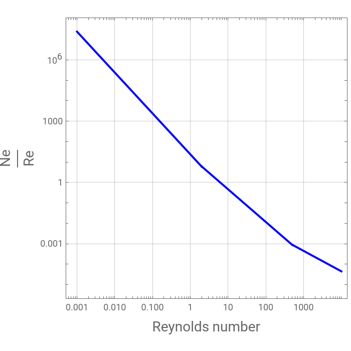
Plotting the Newton Number divided by the Reynolds number ( = ) versus the Reynolds number.
Ne
Re
In[]:=
plt3=LogLogPlot[x]x,{x,10^-3,10^4},PlotRangeAll,PlotPoints10000,GridLinesAutomatic,PlotStyle{Thick,RGBColor[0,0,1]},FrameTrue,AspectRatio->1,ImageSize->350{1,1},FrameLabel->Style["Reynolds number",14],Style"",14
N
e
Ne
Re
Out[]=
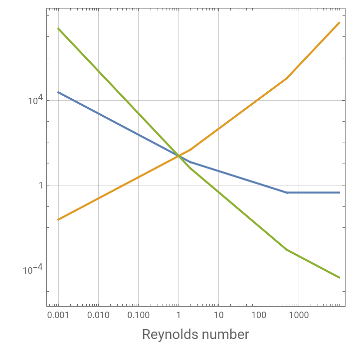
The three plots have a common intersection point.
In[]:=
LogLogPlot{[x],[x]x^2,[x]/x},{x,10^-3,10^4},PlotRangeAll,PlotPoints10000,GridLinesAutomatic,PlotStyleThick,FrameTrue,AspectRatio->1,ImageSize->350{1,1},FrameLabel->{Style["Reynolds number",14],Style["",14]},PlotLegends->LineLegendAutomatic,"Newton number","Archimedes number",""
N
e
N
e
N
e
Ne
Re
Out[]=


Turbulent case:
tfv is the terminal fall velocity. Expression of the tfv depends on the flow type.
Dp is particle diameter. η is the fluid's viscosity. ρ1 is the fluid's density. ρ2 is the spherical particle density. g is the gravitational acceleration. Ar is the Archimedes number.
tfv is the terminal fall velocity. Expression of the tfv depends on the flow type.
Dp is particle diameter. η is the fluid's viscosity. ρ1 is the fluid's density. ρ2 is the spherical particle density. g is the gravitational acceleration. Ar is the Archimedes number.
In[]:=
η=1.410^-3;Dp=510^-3;ρ2=1260;ρ1=1042;g=9.81;
In[]:=
A
r
Out[]=
189490.
In[]:=
sol1=FindRoot[[x]x^2,{x,500}]
A
r
N
e
Out[]=
{x648.913}
In[]:=
tfv[Re_]:=IfRe<2,1(18η)Dp^2Abs[ρ2-ρ1]g,IfRe<500,Reη(Dpρ1),
3Abs[ρ2-ρ1]Dpg
ρ1
In[]:=
tfv[x/.sol1]
Out[]=
0.175459
Laminar case: tfv is the terminal fall velocity. Expression of the tfv depends on the flow type. For laminar flow, tfv is given by Stokes' law.Dp is particle diameter. η is the fluid's viscosity. ρ1 is the fluid's density. ρ2 is the spherical particle density. g is the gravitational acceleration.
In[]:=
η=1.6810^-3;Dp=1.010^-6;ρ2=916;ρ1=1033;g=9.81;
In[]:=
A
r
Out[]=
5.60113×
-7
10
In[]:=
sol2=FindRoot[[x]x^2,{x,500}]
A
r
N
e
Out[]=
{x2.3338×}
-8
10
In[]:=
tfv[Re_]:=IfRe<2,1(18η)Dp^2Abs[ρ2-ρ1]g,IfRe<500,Reη(Dpρ1),
3Abs[ρ2-ρ1]Dpg
ρ1
In[]:=
tfv[x/.sol2]
Out[]=
3.79554×
-8
10
Transition case:
tfv is the terminal fall velocity. Expression of the tfv depends on the flow type.
Dp is particle diameter. η is the fluid's viscosity. ρ1 is the fluid's density. ρ2 is the spherical particle density. g is the gravitational acceleration.
tfv is the terminal fall velocity. Expression of the tfv depends on the flow type.
Dp is particle diameter. η is the fluid's viscosity. ρ1 is the fluid's density. ρ2 is the spherical particle density. g is the gravitational acceleration.
In[]:=
η=1.6810^-2;Dp=1.010^-2;ρ2=916;ρ1=1033;g=9.81;