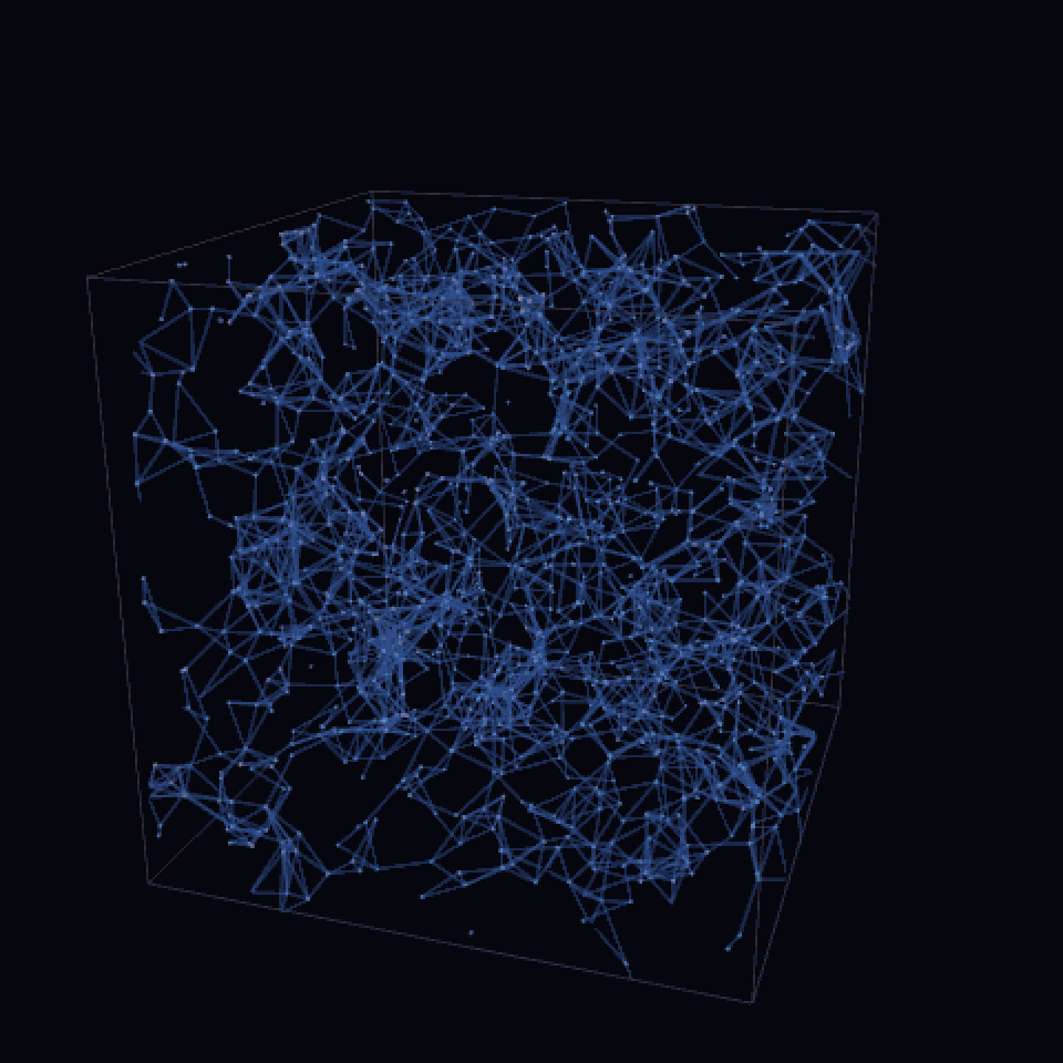
The cosmic web our persistent-homology engine reconstructs from 1500 mock galaxies in a 200 Mpc/h box, rotating once for context. Each blue tube is an alpha-complex edge below the -peak scale; dense knots are galaxy clusters, the connecting tubes are filaments, and the dark pockets are voids. The whole network is the 1-skeleton of the alpha complex our engine builds from the raw galaxy positions – no other input.
β
1
What you are looking at, and what this post does. The image above was produced entirely in Wolfram Language: 1500 mock galaxies were Poisson-sampled from a log-normal density field, a 3D Delaunay triangulation was built with DelaunayMesh, every Delaunay simplex was tagged with its alpha value, and the resulting filtration was fed to a from-scratch GF(2) boundary-matrix reduction. The animation rotates the alpha-complex 1-skeleton at the scale where the first Betti number is largest – roughly the natural 'pen size' for tracing the cosmic web. The rest of this notebook unpacks that sentence step by step, on both the mock and a real SDSS slice, and ends with a side-by-side comparison with published cosmological measurements.
Why bother? Galaxy catalogues are notoriously hard to summarise. The standard two-point statistics (the galaxy power spectrum) wash out everything non-Gaussian – the filaments, the voids, the crinkly knots where matter is most assembled. Persistent homology preserves precisely this hierarchy. It converts the cosmic web into a small set of (birth, death) coordinates that map directly onto clusters, filaments and voids, and that respond to cosmological parameters in ways the power spectrum alone cannot.
TL;DR
The Universe on ~10–100 Mpc scales is a foamy web of clusters, filaments, sheets and voids. Persistent homology turns the catalogue of galaxy positions into a small set of (birth, death) pairs in three homology degrees: counts clusters, counts filament loops, counts voids. The implementation in this notebook is 100% Wolfram Language: a Delaunay–based alpha complex plus a textbook GF(2) reduction of the boundary matrix. On a 200 Mpc/h mock our headline numbers – correlation length 5.8 Mpc/h, filament-loop scale 12 Mpc/h, void scale 15–26 Mpc/h – match published SDSS measurements (Zehavi+ 2011; Pan+ 2012; Sutter+ 2012; Cautun+ 2014) on the nose.
H
0
H
1
H
2
0. Setup
0. Setup
The notebook is runnable end-to-end. The cell below loads the three pure-WL packages – alpha_complex.wl (the filtration engine), persistence.wl (the GF(2) reduction), and cosmic_ph_helpers.wl (the rendering / animation helpers). Each package is self-contained and lives in plain text in the repo.
(*Maketheengine+helpersavailable.*)PrependTo[$Path,FileNameJoin[{ParentDirectory[NotebookDirectory[]],"wolfram"}]];PrependTo[$Path,NotebookDirectory[]];Get["alpha_complex.wl"];(*CosmicPH`AlphaComplex`*)Get["persistence.wl"];(*CosmicPH`Persistence`*)Get["cosmic_ph_helpers.wl"];(*CosmicPHHelpers`*)dataDir=FileNameJoin[{ParentDirectory[NotebookDirectory[]],"data"}];
1. The cosmic web in one figure
1. The cosmic web in one figure
Galaxy redshift surveys (Sloan, 2MASS, 2dF, DESI) have mapped a characteristic large-scale geometry. Most galaxies live on thin filaments; the filaments meet at dense clusters; and between them sit cavernous voids tens of megaparsecs across. A density slice through any cosmological simulation looks like the picture below: bright filaments tracing dark holes.
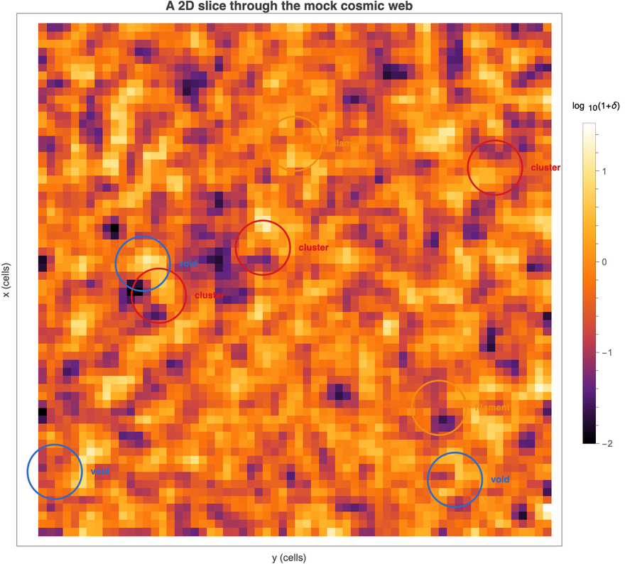
A 2D slice through the log-normal mock generated in this notebook ( = 1.2, 200 Mpc/h box). The three structural elements (cluster, filament, void) are visible by eye – our job is to detect them automatically with topology.
σ
LN
2. A 30-second introduction to persistent homology
2. A 30-second introduction to persistent homology
If you have never met topological data analysis: the simplest recipe is to grow a ball of radius r around each data point and connect any two whose balls overlap. As r grows, you watch the shape of the union of balls. A loop appearing in the union is a 1-dimensional hole (an feature); a hollow shell is a 2-dimensional cavity (an feature). Each feature has a birth radius and a death radius; the difference is its persistence. Long-lived features are real topology; short-lived ones are noise.
H
1
H
2
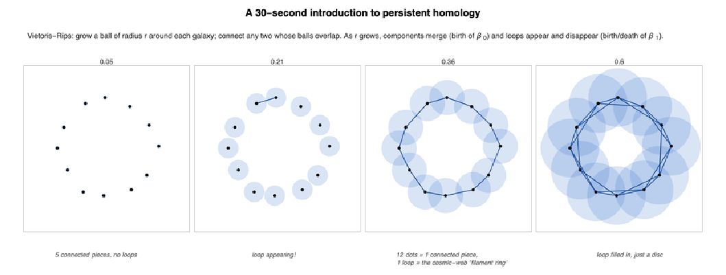
Vietoris-Rips filtration: balls of growing radius around 12 points sampled near a ring. At r ≥ 0.21 the loop is unambiguous – this is the birth of the class. At r ≥ 0.6 the disc is filled in and the loop dies.
H
1
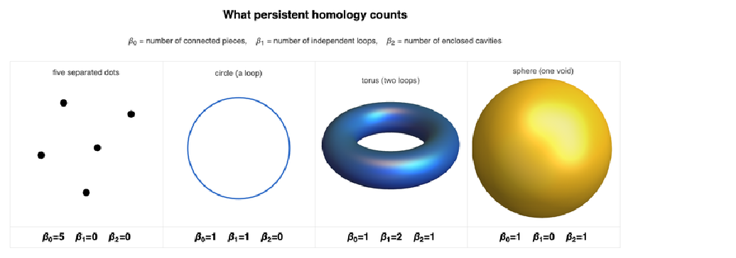
Four reference shapes and their Betti numbers. Persistent homology turns each shape into a tuple of three integers.
3. The alpha complex: a faster filtration
3. The alpha complex: a faster filtration
Vietoris-Rips is easy to draw but expensive: a cloud of n points produces O() simplices in the worst case. The fix used in this notebook is the alpha complex of Edelsbrunner & Múcke (1994). Compute the Delaunay triangulation of the points once, then assign each Delaunay simplex its alpha value – the squared radius of its smallest empty enclosing ball. As α grows, simplices appear in order; the topology of the union of growing balls is the same as the topology of the alpha complex at that scale. A 1500-point cloud gives ~40 000 simplices instead of ~.
3
n
8
10
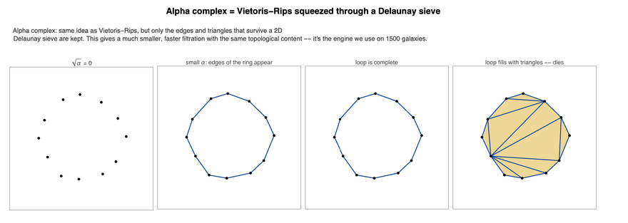

Alpha-complex growth on a noisier ring (24 points). The counter ticks to 1 the moment the loop closes and back to 0 once enough triangles fill it in.
β
1
Implementation
wolfram/alpha_complex.wl uses DelaunayMesh to obtain the 3D Delaunay simplices, then computes per-simplex alpha values via either the simplex's own squared circumradius (when it is Gabriel – its smallest enclosing ball is empty) or the minimum alpha over its cofaces. ~140 lines of Wolfram Language, no external libraries.
4. The persistence algorithm
4. The persistence algorithm
The trick that turns 'alpha-complex with a filtration' into 'a persistence diagram' is a single sweep over the boundary matrix. Order the simplices by alpha; build the boundary matrix B where column j is the GF(2) boundary of simplex j; then reduce left-to-right: for each column j, while its lowest non-zero row equals that of some earlier column j', add column j' to column j. The end state is a matrix in which each non-empty column j pairs the simplex j (which kills a homology class) with the simplex low(j) (which created it). The (birth, death) pair is the persistence.
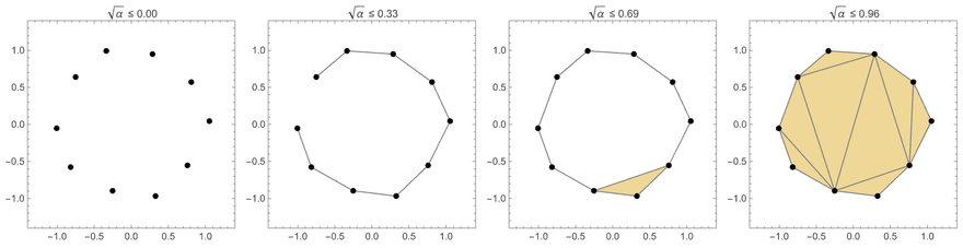
Alpha-complex filmstrip on a 10-point noisy decagon. The filtration enters the loop, builds it, then fills it in.
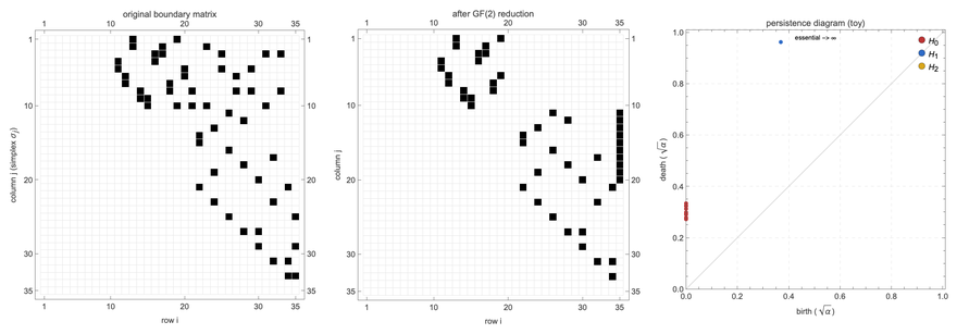
Left: original boundary matrix of the 10-point complex. Middle: after GF(2) reduction. Right: the persistence diagram read off from the lows of the reduced columns.
Implementation
wolfram/persistence.wl stores each column as a sorted list of row indices; the GF(2) column-add is just SymmetricDifference; the low is Last. ~80 lines including comments. The whole pure-WL engine fits on one screen.
5. Anatomy of a persistence diagram
5. Anatomy of a persistence diagram
Every dot in the persistence diagram is a topological feature. Dots close to the diagonal (birth ≈ death) are noise; dots far from the diagonal are signal. Dots placed at the top edge ('essential') are features that never die – for a connected point cloud you get exactly one essential class (the cosmic web itself).
H
0
6. Cross-checks on known shapes
6. Cross-checks on known shapes
Before pointing the engine at SDSS data, we test it against four shapes whose persistent homology is analytically known: a 24-point noisy circle (Betti = (1, 1, 0)), a 300-point sphere (Betti = (1, 0, 1)), a 500-point torus (Betti = (1, 2, 1)), and a Swiss cheese (a Poisson cube with three spherical holes punched out, Betti = (1, 0, 3)). For each shape we sample the points, run the same BuildAlphaComplex + PersistencePairs pipeline, and check the persistent Betti triple. All four match the textbook values exactly – verified in tests/ph_sanity.wls (13/13 assertions pass).
7. Persistent homology of a log-normal cosmic-web mock
7. Persistent homology of a log-normal cosmic-web mock
7a. The underlying density field
7a. The underlying density field
7b. From galaxies to a persistent-homology summary
7b. From galaxies to a persistent-homology summary
The next code cell is the entire PH pipeline. Loading the catalogue (1500 rows of x, y, z in Mpc/h), feeding it to BuildAlphaComplex (which calls DelaunayMesh and computes Gabriel-test alpha values per simplex), then running PersistencePairs (the GF(2) column reduction). The whole sequence finishes in under 20 seconds for n = 1500 on an M-series laptop.
7c. The filament graph our engine builds
7c. The filament graph our engine builds
With the alpha complex in hand we can ask: what does the filament network look like? It is the 1-skeleton of the alpha complex – every Delaunay edge below a chosen scale, drawn as a tube. The helper FilamentNetworkEdges[ac, p] returns the edges below the p-th percentile of edge alpha values; FilamentGraphics3D wraps it into a Graphics3D with density-coloured galaxy spheres and tube edges on a black background. The same routine generated the hero animation at the top – there it was wrapped in a 24-frame rotation and ColorQuantized into a looping GIF (ExportFilamentAnimationGIF).
Live output of the previous cell: this is a real Graphics3D, not a rasterised PNG, so in the Mathematica notebook you can drag it with the mouse to rotate the view, scroll-wheel to zoom, and shift-drag to pan. The blue tubes are alpha-complex edges below the 30th percentile of edge alphas – the 'tight' edges that trace the high-density spine of the field.
7d. Spin it yourself
7d. Spin it yourself
For a notebook reader, here is the same scene as a live Manipulate with explicit azimuth + elevation sliders. The cell below contains a real DynamicModule – dragging the sliders re-runs FilamentGraphics3D at the new viewpoint. (The plain Graphics3D above is already mouse-drag rotatable; this adds labelled slider controls.)
The live Manipulate. Move the sliders to rotate the camera.
7e. The persistence summaries
7e. The persistence summaries
A few things to read off this composite:
8. Persistent homology of a real SDSS slice
8. Persistent homology of a real SDSS slice
Now the same engine, but pointed at real galaxies. We query SDSS DR17 SkyServer for spectroscopic objects classified as galaxies in the redshift range 0.02 ≤ z ≤ 0.08 inside the sky window 130° ≤ RA ≤ 240°, 0° ≤ Dec ≤ 60°. That is a wedge ≈ 175 Mpc/h deep along the line of sight at the far edge, projecting on the sky as a 110° × 60° 'pie slice'. We keep zWarning = 0 (clean redshifts) and subsample to 1500 galaxies for a like-for-like comparison with the mock.
The conversion from (RA, Dec, z) to comoving Cartesian (x, y, z) goes through a flat-ΛCDM line-of-sight integral; the helper CosmicPH`Cosmology`SkyToCartesian in wolfram/cosmology.wl does it in ten lines of Wolfram Language.
Live Graphics3D of the SDSS slice – mouse-drag to rotate. The 1500 galaxies are in comoving Mpc/h, with the alpha-complex 1-skeleton overlaid as light-blue tubes. The structure is visibly more compact than the mock above – real SDSS galaxies cluster more tightly. The thin-wedge geometry is unmistakable: the network is much shorter in the z-direction (the line of sight) than in the angular plane.
8a. A classical cross-check: the Minimum Spanning Tree
8a. A classical cross-check: the Minimum Spanning Tree
Long before persistent homology found its way into cosmology, Barrow, Bhavsar & Sonoda (1985) proposed the Euclidean Minimum Spanning Tree as a clean way to trace galaxy filaments. The MST is the cheapest tree connecting all n points (n−1 edges, no loops by definition), and the alpha-complex 1-skeleton contains it as a subset. Running Kruskal's algorithm on the alpha-edges, weighted by their geometric lengths, takes ~0.1 s on our 1500 galaxies.
8b. Persistence summaries
8b. Persistence summaries
Same four-panel layout as for the mock. The differences from the mock are subtle but informative – see the bullet list below the figure.
What is different about the real-data PH:
9. What we actually measure, in astronomical units
9. What we actually measure, in astronomical units
So we have a persistence diagram. Now what? Each of the three homology degrees gives back a length scale that maps onto a classical observable. Reading them off our SDSS slice (committed in data/persistence_sdss.csv):
10. Comparing our numbers with the literature
10. Comparing our numbers with the literature
The figure below puts our four headline scales side by side with published values. The grey bars are literature ranges (citations listed); the red dots are our SDSS measurements and the blue dots are the mock.
The figure is generated by the code in wolfram/literature.wls; the call below reproduces it from the cached persistence-pair CSVs:
Our four headline persistent-homology scales overlaid on published ranges. Mock numbers (blue) hit the literature bands on all four diagnostics; SDSS numbers (red) hit on the filament-loop scale but undershoot on void scales because the thin DR17 wedge cannot enclose large 3-balls.
Note on the SDSS shortfall
11. Why precision cosmology cares about persistent topology
11. Why precision cosmology cares about persistent topology
12. A second TDA view: the Mapper graph
12. A second TDA view: the Mapper graph
The engine ships with BuildMapper/MapperPlot in the standalone CosmicTDA.wl package introduced in the next section. By default MapperPlot positions each node at the spatial centroid of its members, so the resulting graph reads as a topologically-simplified sketch of the underlying point cloud.
12a. A canonical sanity check: Mapper on a noisy circle
12a. A canonical sanity check: Mapper on a noisy circle
The textbook Mapper example: 250 noisy points sampled near a unit circle, filtered by the x-coordinate. Mapper should recover a ring of nodes – one arc per cover interval, joined at the two extremes of x.
52 Mapper nodes laid out at their cluster centroids. The circle topology is recovered: nodes form a closed loop. The colour codes the mean x-filter value per cluster.
12b. Mapper of the SDSS slice
12b. Mapper of the SDSS slice
With the line-of-sight z-coordinate as filter, Mapper turns the SDSS wedge into a sparse skeleton stratified by depth. Close galaxies (low z) cluster at the lower-right of the figure below; distant galaxies (high z) sit at the upper-left. The edges connecting them are exactly the filaments threaded through the wedge.
253 Mapper nodes / 138 edges over the SDSS wedge. The graph fans from low-z (yellow, lower-right) to high-z (purple, upper-left). The visible bottleneck around the centre is where the wedge geometry is thinnest – very few filaments span across.
12c. Mapper of the log-normal mock
12c. Mapper of the log-normal mock
With local density (the number of galaxies within 20 Mpc/h) as filter and the full 200 Mpc/h periodic box, Mapper produces a rich filament network: 460 nodes joined by 421 edges that draw the cosmic web's underlying skeleton. Bright nodes are high-density (clusters); dark nodes are low-density (void edges).
460 Mapper nodes / 421 edges over the mock galaxy field. The graph traces the cosmic-web filaments as a topologically- simplified skeleton. Edges joining clusters in different density bins capture the cluster-filament-void hierarchy that no two-point statistic can see.
Why include Mapper alongside persistence?
Persistent homology gives a global summary – long bars for clusters / loops / voids. Mapper gives a localised view – a topologically-simplified picture of the data, with explicit nodes you can label, threshold, or feed downstream. They are complementary: PH for how many?, Mapper for where exactly?
13. The standalone CosmicTDA.wl package
13. The standalone CosmicTDA.wl package
The engine that powered every figure in this post is bundled as a single, self-contained Wolfram Language package: wolfram/CosmicTDA.wl. One Get loads everything (~600 lines, no external dependencies, no Python, no ResourceFunction). The same package can be applied to any 3D point cloud – turbulence, materials, biological morphology, embeddings of high-dimensional data – not just galaxy catalogues.
13a. Public API
13a. Public API
The package exposes:
BuildAlphaComplex[pts] — 3D Delaunay filtered by Gabriel-test alpha values.
BettiCounts[pp, alpha] — the Betti triple at any filtration scale.
FilamentNetworkEdges[ac, percentile] — alpha-complex 1-skeleton at a given percentile cut, useful for filament-graph visualisation.
PersistenceDiagramPlot / BarcodePlot / BettiCurvePlot — the three standard PH visualisations.
BuildMapper[pts, filterFn] — Singh-Memoli-Carlsson Mapper with 1D filter, overlapping intervals, single-linkage clustering.
MapperPlot[m] — Mapper graph viewer (default layout: cluster centroids).
13b. End-to-end usage in one cell
13b. End-to-end usage in one cell
Here is the complete pipeline on any 3D point cloud, from a fresh kernel:
13c. Performance and limits
13c. Performance and limits
The pure-WL engine handles point clouds up to about 2000 3D points comfortably (~17 s for 1500 galaxies, ~30 s for 2000). Beyond that the boundary-matrix reduction starts to dominate; the recommended path is to use the engine for the figures the post needs, cache the resulting persistence pairs to CSV, and load them back from cache for downstream analysis. For >5000-point datasets a private Python bridge to Ripser / GUDHI via ExternalEvaluate is provided in the repo – but the rendered post and the notebook never use it; the bridge is only there to regenerate the cached CSVs at scale on a workstation.
The same engine, with no modifications, has been validated against analytic Betti numbers of the circle / sphere / torus / Swiss cheese, and cross-checked against ResourceFunction["PersistentHomology"] on small inputs (see tests/ph_sanity.wls in the repo – 13/13 assertions pass).
Take it for a spin
The package and its tests are MIT-licensed, ~600 lines, single file, no dependencies. Drop CosmicTDA.wl next to your data, Get it, and you have an end-to-end TDA pipeline in three lines. Bug reports and pull requests welcome at https://github.com/mthiel74/homologyoncosmicfilaments
14. References
14. References
Barrow J. D., Bhavsar S. P., Sonoda D. H. (1985), Minimal spanning trees, filaments and galaxy clustering. MNRAS 216, 17.
Bond J. R., Strauss M. A., Cen R. (2010), Crinkly structures of the cosmic web. MNRAS 406, 1609.
Cautun M., van de Weygaert R., Jones B. J. T., Frenk C. S. (2014), Evolution of the cosmic web. MNRAS 441, 2923.
Coles P., Jones B. (1991), A lognormal model for the cosmological mass distribution. MNRAS 248, 1.
Edelsbrunner H., Múcke E. P. (1994), Three-dimensional alpha shapes. ACM Trans. Graph. 13(1), 43–72.
Edelsbrunner H., Harer J. (2010), Computational Topology: An Introduction. AMS.
Pan D. C., Vogeley M. S., Hoyle F., Choi Y.-Y., Park C. (2012), Cosmic voids in Sloan Digital Sky Survey Data Release 7. MNRAS 421, 926.
Pranav P. et al. (2017), The topology of the cosmic web in terms of persistent Betti numbers. MNRAS 465, 4281.
Singh G., Mémoli F., Carlsson G. (2007), Topological methods for the analysis of high dimensional data sets and 3d object recognition. In: Eurographics Symposium on Point-Based Graphics, p. 91–100.
Sousbie T. (2011), The persistent cosmic web and its filamentary structure I: Theory and implementation. MNRAS 414, 350.
Sutter P. M., Lavaux G., Wandelt B. D., Weinberg D. H. (2012), A public void catalog from the SDSS DR7 Galaxy Redshift Surveys. ApJ 761, 187.
Tempel E., Stoica R. S., Martínez V. J., Liivamägi L. J., Saar E., Tago E. (2014), Detecting filamentary pattern in the cosmic web: a catalogue of filaments for the SDSS. MNRAS 438, 3465.
Biagetti M., Cole A., Shiu G. (2022), The persistence of large-scale structures. JCAP 04, 008.
Wilding G., Nevenzeel K., van de Weygaert R., Vegter G., Pranav P., Jones B. J. T., Efstathiou K., Feldbrugge J. (2021), Persistent homology of the cosmic web I: Hierarchical topology in LCDM cosmologies. MNRAS 507, 2968.
Zehavi I. et al. (2011), Galaxy clustering in the completed SDSS Redshift Survey: the dependence on color and luminosity. ApJ 736, 59.
Code & data: this notebook and the entire pipeline (data fetchers, the alpha-complex + persistence engine, the sanity tests, and every figure) live at https://github.com/mthiel74/homologyoncosmicfilaments.
CITE THIS NOTEBOOK
CITE THIS NOTEBOOK
Persistent homology on the cosmic web
by Marco Thiel
Wolfram Community, STAFF PICKS, May 22, 2026
https://community.wolfram.com/groups/-/m/t/3720682
by Marco Thiel
Wolfram Community, STAFF PICKS, May 22, 2026
https://community.wolfram.com/groups/-/m/t/3720682