Original code:
L=10;l=L*(3/1000);DD=0.01;mu=1;sol=ParametricNDSolve[{ϕ1''[s]-(T-F)*Sin[ϕ1[s]]==0,ϕ2''[s]-T*Sin[ϕ2[s]]==0,ϕ1[0]==0,ϕ2'[L]==0,ϕ1[l]==ϕ2[l]==ArcTan[1/mu]},{ϕ1,ϕ2},{s,0,L},{T,F}];m1[s_,T_,F_]:=Evaluate[Evaluate[ϕ1[T,F]/.sol][s]];m2[s_,T_,F_]:=Evaluate[Evaluate[ϕ2[T,F]/.sol][s]];dm1[s_,T_,F_]:=Evaluate[D[m1[s,T,F],s]];dm2[s_,T_,F_]:=Evaluate[D[m2[s,T,F],s]];BC1[T_?NumericQ,F_?NumericQ]:=NIntegrate[Cos[m1[s,T,F]],{s,0,l}]-DD;BC2[T_?NumericQ,F_?NumericQ]:=-dm1[l,T,F]+dm2[l,T,F];sol2=Monitor[FindRoot[{BC1[T,F]==0,BC2[T,F]==0},{{T,1},{F,1}}],{T,F}]
Here are calculated separately, which is hopefully faster:
ϕ1,ϕ2
In[]:=
Clear[solPhi1,m1,m2,dm1,dm2,BC1,BC2,T,F,s,intCos,ϕ1,ϕ2];L=10;l=L*(3/1000);DD=1/100;mu=1;solPhi1=ParametricNDSolve[{ϕ1''[s]-(T-F)*Sin[ϕ1[s]]==0,intCos'[s]==Cos[ϕ1[s]],ϕ1[0]==0,ϕ1[l]==ArcTan[1/mu],intCos[0]==0},{ϕ1,intCos},{s,0,l},{T,F}];solPhi2=ParametricNDSolve[{ϕ2''[s]-T*Sin[ϕ2[s]]==0,ϕ2'[L]==0,ϕ2[l]==ArcTan[1/mu]},ϕ2,{s,l,L},{T,F},WorkingPrecision->30,MaxSteps->100000];m1[s_,T_,F_]=ϕ1[T,F][s]/.solPhi1;m2[s_,T_,F_]=ϕ2[T,F][s]/.solPhi2;dm1[s_,T_,F_]=ϕ1[T,F]'[s]/.solPhi1;dm2[s_,T_,F_]:=dm2[s,T,F]=ϕ2[T,F]'[s]/.solPhi2;BC1[T_,F_]=intCos[T,F][l]-DD/.solPhi1;BC2[T_,F_]=-dm1[l,T,F]+dm2[l,T,F];
Here I show a solution of the first equation . The second equation is too hard, at least for me.
BC1[T,F]==0
BC2[T,F]==0
The equation for ϕ1
The equation for
ϕ1
Since only depends on , the equation is equivalent to . We can try to solve it independently of .
ϕ1
T-F
BC1[T,F]==0
BC1[0,F-T]==0
ϕ2
Here is a plot of :
BC1[0,FminusT]
In[]:=
Plot[BC1[0,FminusT],{FminusT,0,12000},PlotLabel->"function BC1"]
Out[]=
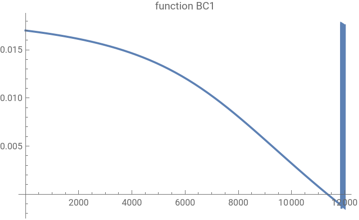
We see it has a probem when is near 12000. Luckily, it crosses the level 0 before that, near .
FminusT
FminusT==11000
Let us zoom in:
In[]:=
Plot[BC1[0,FminusT],{FminusT,11000,11500},PlotLabel->"function BC1"]
Out[]=
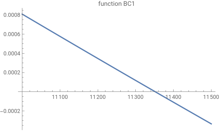
To approximate the solution better, let us try FindRoot:
In[]:=
FindRoot[BC1[0,FminusT]==0,{FminusT,11300}]solFminusT=FminusT/.%BC1[0,solFminusT]
Out[]=
{FminusT11351.7}
Out[]=
11351.7
Out[]=
2.77556×
-17
10
Confirmation that we have indeed a solutio, from a different route:
In[]:=
NIntegrate[Cos[m1[s,0,solFminusT]],{s,0,l}]-DD
Out[]=
2.15989×
-9
10
It is not guaranteed that this is the only solution.
solFminusT
The function corresponding to this value of seems to satisfy the boundary conditions to a high enough precision:
ϕ1
FminusT
In[]:=
m1[0,0,solFminusT]{m1[l,0,solFminusT],Pi/4//N}
Out[]=
-9.2293×
-8
10
Out[]=
{0.785398,0.785398}
The slope of at the point is
ϕ1
s==l
In[]:=
slopeϕ1=dm1[l,0,solFminusT]
Out[]=
-132.27
Here is a plot of :
ϕ1
In[]:=
Plot[m1[s,0,solFminusT],{s,0,l},GridLines->{{l},{Pi/4}},PlotLabel->"function ϕ1",Epilog->{PointSize[Medium],Point[{0,0}],Point[{l,Pi/4}],Dashed,InfiniteLine[{l,Pi/4},{1,slopeϕ1}]}]
Out[]=
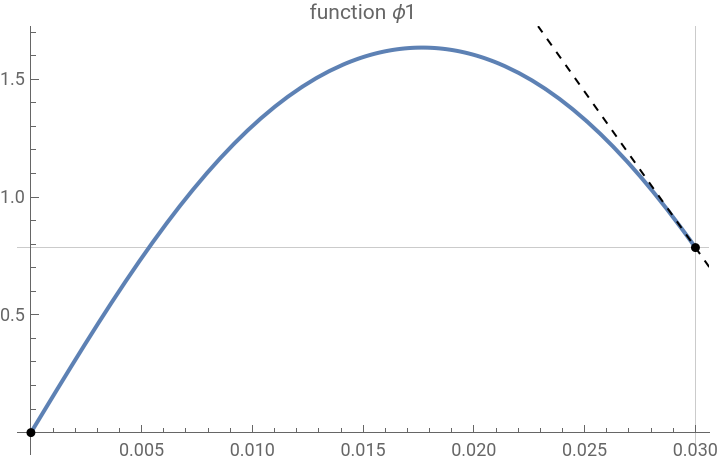
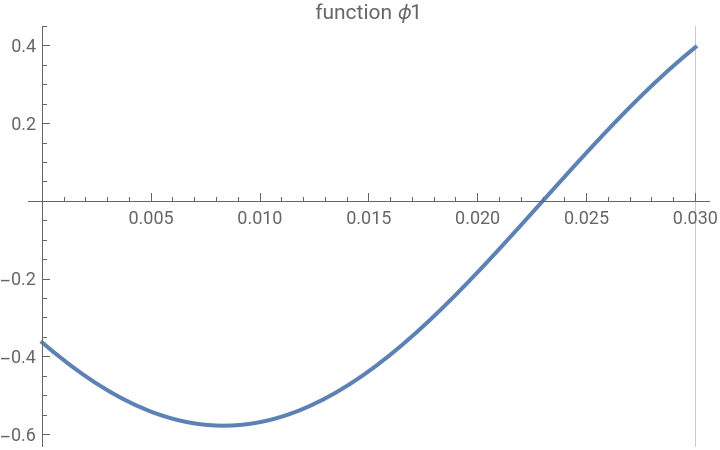
We cannot trust the numerical solutions when is larger than about , at least with the default settings. The function corresponding to is plotted here, and it does not satisfy the boundary conditions at all:
FminusT
12000
ϕ1
FminusT=12000
In[]:=
Plot[m1[s,0,12000],{s,0,l},GridLines->{{l},{Pi/4}},PlotLabel->"function ϕ1"]
Out[]=
The equation for ϕ2
The equation for
ϕ2
The equations can be rewritten as
BC1[T,F]==0,BC2[T,F]==0
BC1[T,F]==0&&BC2[T,F]==0BC1[0,F-T]==0&&BC2[T,F]==0
We have already found a solution for , where . Assuming that solution, we can rewrite the second equation:
BC1[0,F-T]==0
F-T=solFminusT
BC2[T,F]==0-dm1[l,T,F]+dm2[l,T,F]==0-dm1[l,0,F-T]+dm2[l,T,0]==0-dm1[l,0,solFminusT]+dm2[l,T,0]==0-slopeϕ1+dm2[l,T,0]==0-slopeϕ1+ϕ2'[l]==0ϕ2'[l]==slopeϕ1
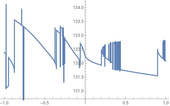
Here is a plot of for between and 1:
-slopeϕ1+dm2[l,T,0]
T
-1
Plot[-slopeϕ1+dm2[l,T,0],{T,-1,1}]
Out[]=
Conclusion
Conclusion