OrthogonalTrayectories::usage="When all the curves in a family G(x, y, ) = 0 intersect orthogonally with all the curves of the other family H(x, y, ) = 0, the families are said to be orthogonal trajectories of each other. If = f(x, y) it's the differential equation of a family, then the differential equation for the orthogonal trajectories of this family will be = - . Find the orthogonal trajectories for the family y = References: Zill, D.G., Cullen, M.R. Differential Equations with Boundary-Value Problems. Ed. Brooks/Cole: p.80, 1977.";
c
1
c
2
y
x
y
x
1
f(x,y)
1
(x+)
c
1
Development:
xy+y=1
c
1
We derive implicity with respect to x:
x+y+=0;=-;
y
x
c
1
y
x
y
x
y
x+
c
1
From the original equation we clear and we substitute it in the differential equation:
c
1
c
1
1
y
y
x
y
x+-x
1
y
y
x
2
y
We look for the orthogonal trajectories, then:
y
x
1
2
y
In[]:=
DSolvey'[x]==1,y[x],x
2
(y[x])
Out[]=
y[x]-,y[x],y[x]
1/3
(-3)
1/3
(x+)
1
1/3
3
1/3
(x+)
1
2/3
(-1)
1/3
3
1/3
(x+)
1
We take one of the solutions and raise it to the cube:
3
y
c
2
In[]:=
ContourPloty==,==3x-5,y==,==3x-4,y==,==3x-3,y==,==3x-2,y==,==3x-1,y==,==3x,y==,==3x+1,y==,==3x+2,y==,==3x+3,y==,==3x+4,y==,==3x+5,{x,-5,5},{y,-5,5},AxesTrue,AxesOrigin{0,0},BoxRatiosAutomatic,PlotRangeAll,PerformanceGoal"Quality"
1
x-5
3
y
1
x-4
3
y
1
x-3
3
y
1
x-2
3
y
1
x-1
3
y
1
x
3
y
1
x+1
3
y
1
x+2
3
y
1
x+3
3
y
1
x+4
3
y
1
x+5
3
y
Out[]=
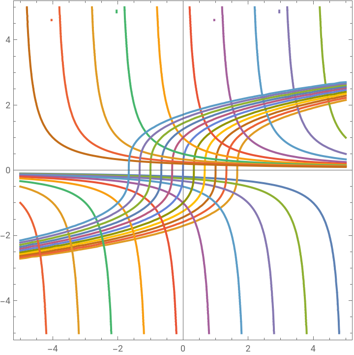
In[]:=
NSolvey==,==3x-2,{x,y}
1
x-2
3
y
Out[]=
{{x2.56043,y1.78436},{x1.77514+0.601106,y-0.545927-1.45938},{x1.77514-0.601106,y-0.545927+1.45938},{x0.555967,y-0.692505}}
In[]:=
δ=ResourceFunction["TangentLine"]y==,{x,2.560425660450319},y,"Plot";ζ=ResourceFunction["TangentLine"][==3x-2,{x,2.560425660450319},y,"Plot"];Show[δ,ζ]
1
x-2
3
y
Out[]=
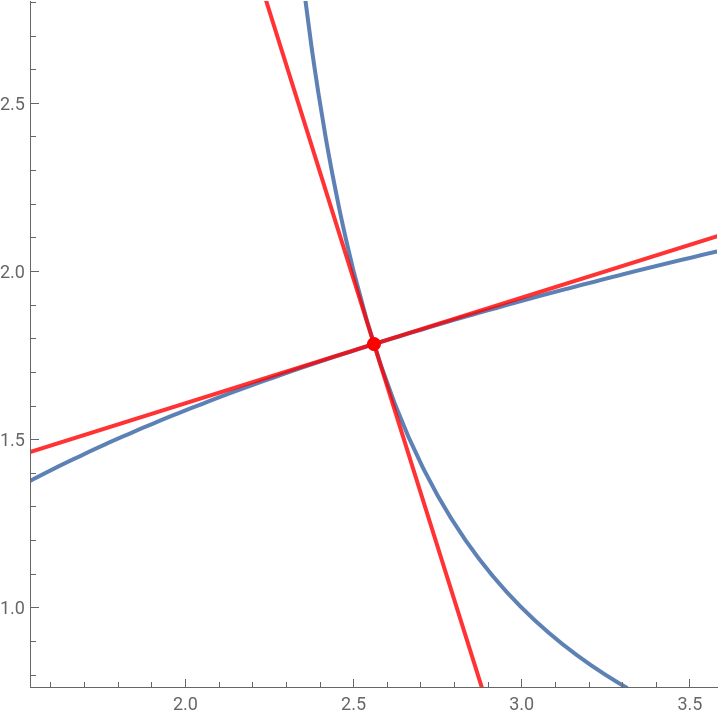
This graph shows at the point {2.56043, 1.78436} para las curvas con ==-2 clearly because they are called orthogonal trajectories. Their tangent lines at that point are orthogonal to each other.
c
1
c
2
Here are the equations of the tangent lines in each case:
In[]:=
ResourceFunction["TangentLine"]y==,{x,2.560425660450319},y,"SlopeInterceptEquation"
1
x-2
Out[]=
y9.93658-3.18393x
In[]:=
ResourceFunction["TangentLine"][==3x-2,{x,2.560425660450319},y,"SlopeInterceptEquation"]
3
y
Out[]=
y0.980187+0.314077x