Conversion Calculation for Tanks in Series
Authors: Housam Binous and Ahmed Bellagi
Authors: Housam Binous and Ahmed Bellagi
We consider a 50 tanks-in-series case study.
First, second and zero order reactions are treated.
We show how one can obtain the exit concentration and the conversion firstly by solving the system of ordinary differential equations verified by the problem and secondly using RTD given by MacMullin and Weber (see Ref. 1-2) .
References:
1- O. Levenspiel, Chemical Reaction Engineering, 3rd Edition, Wiley, 1999, pages 323.
2- R.B. MacMullin and M. Weber, The Theory of Short-Circuiting in Continuous-Flow Mixing Vessels in Series and Kinetics of Chemical Reactions in Such Systems. Trans. AIChE. 1935; 31(2):409–458.
3- J. J. Carberry, Chemical and Catalytic Reaction Engineering, New York: McGraw Hill, 1976, page 94.
First-order reaction
First-order reaction
Computing conversion using the system of ordinary differential equations that governs the problem.
Mean residence time in a tank is τ. V is the total volume of all tanks. F is the flow rate. Ntanks=50 tanks.
In[]:=
Ntanks=50; V=1; F=0.01;
In[]:=
τ=V/F/Ntanks
Out[]=
2.
Rate constant
In[]:=
k=0.05;
Input concentration of component A
In[]:=
CA
0
Governing Equations
In[]:=
i=2;While[i<Ntanks+1,{eq[i]=D[[t],{t,1}]([t]-[t])/τ-k[t],i++}]
CA
i
CA
i-1
CA
i
CA
i
In[]:=
eq[1]=D[[t],{t,1}]([t]-[t])/τ-k[t];
CA
1
CA
0
CA
1
CA
1
In[]:=
eqn=Table[eq[i],{i,2,Ntanks}];
Eq=Join[{eq[1]},eqn];
Eq=Join[{eq[1]},eqn];
In[]:=
init=Table[[0]0,{i,1,Ntanks}];
CA
i
In[]:=
sys=Join[Eq,init];
In[]:=
Unknown=Table[,{i,1,Ntanks}];
CA
i
computing the exit concentration from each tank.
In[]:=
sol=NDSolve[sys,Unknown,{t,0,1000}];
Plot of the concentration profile at the exit of the last tank
In[]:=
plt1=Plot[[t]/.sol,{t,0,200},PlotStyle{Thick,Darker@Green},PlotRangeAll,AspectRatio1,GridLinesAutomatic,FrameTrue,FrameLabel{Style["time",14],Style["concentration of A @exit",14]},ImageSize400{1,1}]
CA
50
Out[]=
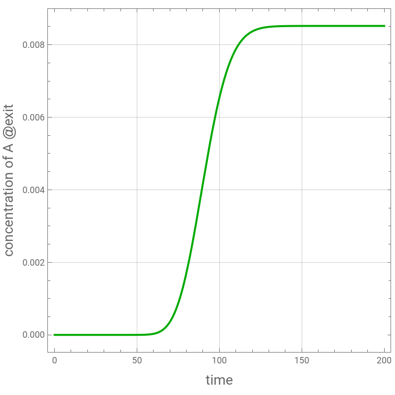
Conversion obtained by solving the system of ODEs and by using the RTD are both equal to 99.15 %.
Conversion (labelled X) is obtained using the steady state value of the exit concentration of the last tank.
In[]:=
X=1-[t]/.sol/.t500//First
CA
50
Out[]=
0.991481
Conversion using the RTD.RTD from MacMullin and Weber’s derivation (1935). 50 tanks case.Also, we have from Ref. 3 with N number of tanks.
X=1-
1
N
(1+kτ)
In[]:=
tbar=Ntanks τ
Out[]=
100.
In[]:=
RTD[t_]:=1/tbar (t/tbar)^(49) 50^50/49! Exp[-50 t/tbar]
In[]:=
X=NIntegrate[RTD[t](1-Exp[-kt]),{t,0,1000}]
Out[]=
0.991481
Derivation of conversion expression given in Ref. 3
Derivation of conversion expression given in Ref. 3
In[]:=
Ntanks=50;k=.;τ=2;tbar=Ntanksτ;
In[]:=
expression=Integrate[1/tbar(t/tbar)^(Ntanks-1)Ntanks^Ntanks/(Ntanks-1)!Exp[-Ntankst/tbar](1-Exp[-kt]),{t,0,Infinity}][[1]]
Out[]=
1-
1
50
(1+2k)
In[]:=
Ntanks=50;k=0.05;τ=2;
In[]:=
X=1-1/(1+kτ)^Ntanks(*fromRef.3*)
Out[]=
0.991481
Zero-order reaction
Zero-order reaction
Computing conversion using the system of ordinary differential equations that governs the problem.
Mean residence time in a tank is τ. V is the total volume of all tanks. F is the flow rate. Ntanks=50 tanks.
In[]:=
Ntanks=50; V=1; F=0.01;
In[]:=
τ=V/F/Ntanks
Out[]=
2.
Rate constant
In[]:=
k=0.0022;
Input concentration of component A
In[]:=
CA
0
Governing Equations. Initially, tanks contain a concentration of component A equal to 1.
In[]:=
i=2;
In[]:=
While[i<Ntanks+1,{eq[i]=D[[t],{t,1}]([t]-[t])/τ-kMax[0,Sign[[t]]],i++}]
CA
i
CA
i-1
CA
i
CA
i
In[]:=
eq[1]=D[[t],{t,1}]([t]-[t])/τ-kMax[0,Sign[[t]]];
CA
1
CA
0
CA
1
CA
1
In[]:=
eqn=Table[eq[i],{i,2,Ntanks}];
In[]:=
Eq=Join[{eq[1]},eqn];
In[]:=
init=Table[[0]10^-10,{i,1,Ntanks}];
CA
i
In[]:=
sys=Join[Eq,init];
In[]:=
Unknown=Table[,{i,1,Ntanks}];
CA
i
computing the exit concentration from each tank.
In[]:=
sol=NDSolve[sys,Unknown,{t,0,500}];
Plot of the concentration profile at the exit of the last tank
In[]:=
plt2=Plot[[t]/.sol,{t,0,200},PlotStyle{Thick,Darker@Green},PlotRangeAll,AspectRatio1,GridLinesAutomatic,FrameTrue,FrameLabel{Style["time",14],Style["concentration of A @exit",14]},ImageSize400{1,1}]
CA
50
Out[]=
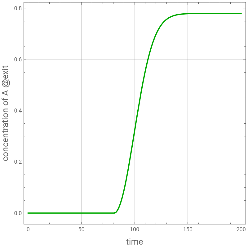
Conversion obtained by solving the system of ODEs and by using the RTD are both equal to 22 %.
Conversion is obtained using the steady state value of the exit concentration of the last tank.
Conversion using the RTD.
RTD from MacMullin and Weber’s derivation (1935). 50 tanks case.
RTD from MacMullin and Weber’s derivation (1935). 50 tanks case.
In[]:=
tbar=Ntanks τ
In[]:=
RTD[t_]:=1/tbar (t/tbar)^(49) 50^50/49! Exp[-50 t/tbar]
Second-order reaction
Second-order reaction
Computing conversion using the system of ordinary differential equations that governs the problem.
Mean residence time in a tank is τ. V is the total volume of all tanks. F is the flow rate. Ntanks=50 tanks.
In[]:=
Ntanks=50; V=1; F=0.01;
Rate constant
In[]:=
k=0.02;
Input concentration of component A
Governing Equations. Initially, tanks contain a concentration of component A equal to 1.
In[]:=
i=2;
In[]:=
eqn=Table[eq[i],{i,2,Ntanks}];
In[]:=
Eq=Join[{eq[1]},eqn];
In[]:=
sys=Join[Eq,init];
computing the exit concentration from each tank.
In[]:=
sol=NDSolve[sys,Unknown,{t,0,5000},AccuracyGoal->20];
Plot of the concentration profile at the exit of the last tank
Conversion obtained by solving the system of ODEs and by using the RTD are both near 66.18 %.
Conversion is obtained using the steady state value of the exit concentration of the last tank.
Conversion using the RTD.
RTD from MacMullin and Weber’s derivation (1935). 50 tanks case.
RTD from MacMullin and Weber’s derivation (1935). 50 tanks case.
In[]:=
tbar=Ntanks τ
In[]:=
RTD[t_]:=1/tbar (t/tbar)^(49) 50^50/49! Exp[-50 t/tbar]