Wolfram Cloud Document

ABSTRACT (original article): Topological band theory based on the variety of reciprocal space invariants provides an insightful framework for quantum material characterization in condensed matter physics. Its bulk–boundary correspondence principle has become a reliable tool for predicting Fermi level properties. Here we investigate a recently proposed bottom-up topological engineering based on reciprocal space invariants and show its connection to a real space in situ topology of a Kekulé structure originating in organic chemistry. We show that these approaches can be effectively used to engineer magnetic-field-free tunable chiral anomalies that are promising for energy-efficient electronic transport. CITATION (original article): Vasil A. Saroka, Victor A. Demin, and Michele Pizzochero, Nano Letters 2026 26 (20), 6532-6540. https://doi.org/10.1021/acs.nanolett.5c06221
Full supplementary files: https://zenodo.org/records/18997300

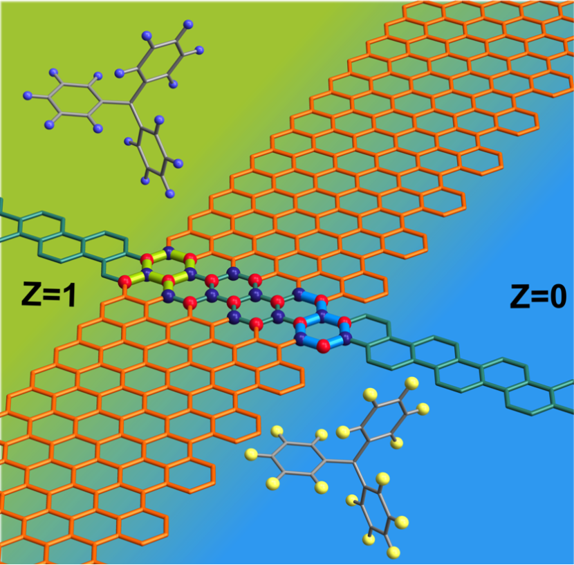
A visual representation of this research was selected as a cover feature for ACS Publications’ Nano Letters (Vol. 26, Issue 20).

In the last two decades, topological band theory has established not only as a useful explanatory framework, but also as a practical tool for materials functionality engineering. Zero-energy modes of carbon nanostructures have been a subject of interest for a long time, and graphene nanoribbons (GNRs) provide a versatile platform for probing and advancing topological engineering of such modes. With the emergence of bottom-up self-assembling methods, it became possible to fabricate nanoribbons in an atomically precise fashion.

This post explores reciprocal space (k-space) defined topological invariants and matchings in the graphs. It covers preparing input data for quantum chemistry and classical molecular dynamics programs.

TBpack and global setting for the current session

Import the requisite TBpack computational modules and configure the overarching global parameters, establishing the precise numerical tolerances and compilation targets essential for accurate theoretical modeling.

In[]:=

ResourceFunction["InstallTBpack"][]

TBpack GitHub page: https://github.com/vasilsaroka/TBpack

Needs["TBpack`"]cdir=NotebookDirectory[];(*RuntimeOptionsglobalsettingforthecurrentsession*)runtimeoptions={"Speed","CatchMachineIntegerOverflow"False,"CompareWithTolerance"False,"EvaluateSymbolically"False};$CompilationTarget="WVM";(*changethisto"WVM"ifyoudonothavesuitableCcompilerinstalled*)<<CCompilerDriver`<<"CompiledFunctionTools`"SetOptions[MaTeX,"Preamble"{"\\usepackage{xcolor}","\\definecolor{darkgreen}{rgb}{0,0.5,0}","\\renewcommand{\\vec}[1]{\\mathbf{\\boldsymbol{#1}}}"}];colordata=ColorData[3,"ColorList"];Grid[Table[{i,colordata〚i〛,(*convertiontoInkscapeRGB*)255List@@(colordata〚i〛)},{i,Length[colordata]}],Background->{None,{{LightBlue,White}}},Dividers->All]

Out[]=

1		{0.,0.,0.}
2		{254.,92.,7.}
3		{254.,252.,9.}
4		{138.,182.,7.}
5		{37.,111.,98.}
6		{2.,130.,237.}
7		{39.,29.,125.}
8		{120.,67.,149.}
9		{227.,3.,125.}
10		{231.,7.,33.}

Functions


Case studies: Nanoribbon analysis with Z invariant and Graphs (29/01/2025)

Apply the established topological and graph-theoretic frameworks to specific Janus nanoribbon geometries, systematically correlating their edge terminations with the anticipated flat band formations.

Scheme 1

Illustrate the overarching paradigm of bottom-up topological band engineering by logically fusing disparate base unit cells into a unified, macroscopic host nanoribbon architecture.

Scheme 1: panel (a)

Visually construct the spatial arrangement of the Janus nanoribbon, emphasizing the distinct crystallographic symmetry and invariant values at the opposing boundaries.

a0=1.42;imax=4;(*Evaluateinitializationcellstosetuczlistvariable!!!*)ruc=uczlist〚1,1〛;Tbase={3a0,0,0};Thost=0,2

a0,0;uc=Join[Flatten[Table[#+(i-1)Tbase&/@ruc,{i,imax}],1],#+(imax)Tbase&/@ruc〚{2,7,4}〛];len=Length[uc](*sortsublattices*)δ1={-a0,0,0};δ2=RotationMatrix[2π/3,{0,0,1}].δ1;δ3=RotationMatrix[2π/3,{0,0,1}].δ2;{uc,sublen}=SublatticeSorting1D[uc,Thost,{δ1,δ2,δ3},"TrackBondsConfiguration"->False];acolor=Flatten[{colordata〚7〛,Table[i->colordata〚10〛,{i,sublen〚1〛}]},1];g=AtomicStructure[{uc,{Thost},a0},AtomColoracolor,BondColorGray,BondSize->0.07,NumberOfUnitCells{5},AtomEnumerationFalse,PlaneProjection->{1,1,1},ImageSize->{300}]

Out[]=

In[]:=

inch=400;(*400pointsinaninch*)imagesize={8.19inch,8.05inch}leuc=uczlist〚1,1〛;reuc=uczlist〚4,1〛;nh=5;LEuc=#+0Tbase+nhThost&/@leuc;REuc=#+(imax-1)Tbase+nhThost&/@reuc;Zl=uczlist〚1,2〛;Zr=uczlist〚4,2〛;(*Herewechangethecolorsforsublatticessothataftermirrorreflectionofthesublattices,theymatchtheoriginalones.ThisisneededbecausemirrorreflectionisusedforpicturedesigninInkscape.*)acolor=Flatten[{colordata〚10〛,Table[i+nhlen->colordata〚7〛,{i,sublen〚1〛}]},1];g=AtomicStructure[{uc,{Thost},a0},AtomColoracolor,AtomSize->Flatten[{0.001,Table[i+nhlen->0.4,{i,Total[sublen]}]}],BondColorDirective[{Opacity[0.9],colordata〚2〛}],BondSize->0.12,NumberOfUnitCells{16},AtomEnumerationFalse,PlaneProjection->{1,1,1},ImageSize->imagesize];acolor=Directive[{Opacity[0.0],White}];gfun=AtomicStructure[{#1,{-Tbase},a0},AtomColoracolor,AtomSize->0.001,BondColorIf[#2!=0,colordata〚4〛,colordata〚6〛],BondSize->0.26,NumberOfUnitCells{1},AtomEnumerationFalse,PlaneProjection->{1,1,1}]&;bruc=Flatten[Table[#+(i-1)Tbase&/@LEuc,{i,Range[-3,10]}],1];gg=AtomicStructure[{bruc,{},a0},AtomColoracolor,BondColorDirective[{Opacity[0.6],colordata〚5〛}],BondSize->0.12,NumberOfUnitCells{},FontSize->7,AtomEnumerationFalse,PlaneProjection->{1,1,1}];fig=Show[{g,gg,MapThread[gfun,{{LEuc,REuc},{Zl,Zr}}]},(*PlotRange->2{-1,1},*)ImageSize->imagesize(*{300}*),PlotRange{{-19.47`,39.35},{-3.76,64.34122},{-2,2}},ViewAngle0.1502,ViewProjection"Perspective",ViewVector{{89.592,-126.759,122.5417},{5.94,25.291,0}},ViewVertical{0,0,1}];

Removing background

Scheme 1: panel (b) - Graph from GNR unit cell

Translate the physical atomic lattice of the nanoribbon into its exact graph-theoretic analog, definitively pinpointing the unmatched vertices responsible for the electronic deficit.

Zigzag orientation

Examine the structural constraints and electronic consequences of engineering host Janus nanoribbons exclusively along the zigzag propagation axis.

Figure 1: panels (b, c, d, e) - Case 8: 1-7

Let's observe the predicted emergence of fully flat bands and the corresponding graph deficit in a representative zigzag host ribbon synthesized from the selected base units.

Armchair orientation

Pivot the analysis to investigate the specific topological phenomena and electronic sub-bands that emerge when host nanoribbons are configured along the armchair direction.

DFT results: 1-7 triarylmethyl edge

Validate the idealized tight-binding models by executing rigorous, first-principles spin-polarized density functional theory calculations on structurally precise, chemically realizable molecular boundaries.

Non-magnetic bands and Figure 3: panel (b) optimized structure [SIESTA]

Calculate the baseline spin-degenerate energy bands from the geometrically optimized lattice, establishing the non-magnetic reference state prior to symmetry breaking.

Figure 3: panel (c) + gif-animation [spin-polarized bands in the external in-plane field; SIESTA]

Trace the dynamic spin-splitting of the electronic bands and document the transition into a definitive chiral anomalous state driven by the application of an external transverse electric field.

Bands in the external in - plane field

Normalized k value

Triple panel figure

Panel 0

Panel 1

Panel 2

.gif-animation of bands in the field

Visual summary

Cover art

Creating the cover art that got featured in ACS Publications: Nano Letters. Bottom-up topological engineering of flat bands in Janus graphene nanoribbons. The base ribbon is depicted in dark green. The host Janus ribbon is depicted in orange. Topological Z invariants are calculated on the unit cells (light green and light blue) of the base ribbon. The triarylmethyl radicals can reinforce host ribbon terminations.

Cover art size:
Image files should be submitted as TIF,JPG,PNG,or EPS files (not PDF or PPT) with a resolution of at least 300 dpi for pixel-based images. Cover art should be 8.19 inches (20.8 cm) wide×8.05 inches (20.45 cm) high at 300 ppi,and submission of “layered” artwork is encouraged. The journal’s logo will obscure the top 2.5 inches (6.35 cm) of the image.