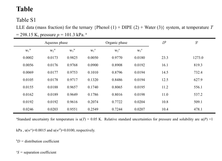
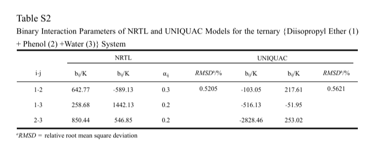
The notebook constructs the full ternary liquid–liquid equilibrium (LLE) diagram for the {Diisopropyl Ether (1) + Phenol (2) + Water (3)} system at T = 298.15 K and P = 1 atm directly from the regressed NRTL binary interaction parameters (Table S2 of Ref. 1), rather than by simply connecting the experimentally measured tie-line endpoints. The goal is to generate a continuous binodal curve and a family of calculated tie lines that can be overlaid on the raw experimental data from Table S1, so that the thermodynamic consistency and predictive quality of the fitted model can be assessed quantitatively through an RMSD comparison rather than just visually.
The starting point is the dimensionless molar Gibbs energy of mixing, gmix[x1,x2] = Σ xᵢ ln(xᵢ) + Σ xᵢ ln(γᵢ), built from the ideal entropy-of-mixing term plus the NRTL excess-Gibbs-energy contribution encoded in lnGamma. This scalar function of two independent mole fractions (with the third fixed by x3 = 1 − x1 − x2) defines a surface over the composition triangle whose curvature governs whether the system is stable as a single phase or splits into two liquid phases.
Two-phase equilibrium between compositions (x1a, x2a) and (x1b, x2b) is thermodynamically equivalent to those two points sharing a common tangent plane on the gmix surface — this is the geometric statement of equal chemical potentials for every component in both phases. Equations eq1–eq5 encode this double-tangent condition explicitly: the partial derivatives dgdx1, dgdx2 must match between the two points (equal slopes in both composition directions), and the tangent-plane values evaluated at each point must coincide (equal intercepts), giving a system of five nonlinear equations in the five unknowns (x1a, x2a, x1b, x2b, plus d which is a Lagrange-type multiplier or slack variable to ensure we avoid the trivial solution).
A direct root-find of this system works only locally; it fails near the plait point, where the two branches of the binodal curve merge and the Jacobian becomes singular (a fold/turning point). To trace the entire curve robustly, the notebook uses pseudo arc-length continuation: an auxiliary normalization equation (auxeq) is appended, requiring the sum of squared derivatives of all unknowns with respect to a new parameter s (arc length along the solution branch) to equal one. This reparameterizes the problem so that s, rather than any single composition variable, advances monotonically even through the fold, and the extra variable d(s) — a measure of the separation between the two coexisting compositions — is tracked so the plait point (if present) can be identified as the point where d → 0.
Numerically, an initial two-phase solution is obtained with FindRoot at s = 0, then the full differential-algebraic system is integrated with NDSolve to produce InterpolatingFunctions for x1a(s), x2a(s), x1b(s), x2b(s) over the accessible arc-length domain. These are used to plot the calculated binodal curve using TernaryListPlot, and calculated tie lines are constructed by matching arc-length positions between the two branches; overlaying the experimental tie lines (given in mass fraction - see Table S1 of Ref. 1) allows direct visual and RMSD-based comparison, yielding a value of about 0.1554.
Together, the common-tangent-plane formulation and the arc-length continuation scheme let the model reproduce not just the eight measured tie lines but the entire theoretical binodal envelope — including the physically delicate region near the plait point (if present) that a parametrization in x1 or x2 alone would not be able to trace continuously.
Together, the common-tangent-plane formulation and the arc-length continuation scheme let the model reproduce not just the eight measured tie lines but the entire theoretical binodal envelope — including the physically delicate region near the plait point (if present) that a parametrization in x1 or x2 alone would not be able to trace continuously.
LLE diagram computation using common tangent plane and arc - length continuation
LLE diagram computation using common tangent plane and arc - length continuation
Parameters at T=298.15 K from my above Table S1
In[]:=
T=298.15;(*K*)
tau_ij for {Diisopropyl Ether (1) + Phenol (2) + Water (3)}
NRTL model-- binary interaction parameters (Table S2)
(*b_ijmatrix(K),rows/colsordered{DIPE,Phenol,Water}*)bNRTL={{0,642.77,258.68},{-589.13,0,850.44},{1442.13,546.85,0}};alphaNRTL={{0,0.3,0.2},{0.3,0,0.2},{0.2,0.2,0}};τ=Table[If[i==j,0,bNRTL[[i,j]]/T],{i,1,3},{j,1,3}];
In[]:=
G[i_,j_]:=Exp[-alphaNRTL[[i,j]]τ[[i,j]]];
Composition vector
In[]:=
xvec[x1_,x2_]:={x1,x2,1-x1-x2};
NRTL activity coefficients
In[]:=
lnGamma[i_,x1_,x2_]:=Module[{x,term1,term2},x=xvec[x1,x2];term1=Sum[x[[j]]τ[[j,i]]G[j,i],{j,1,3}]/Sum[x[[k]]G[k,i],{k,1,3}];term2=Sum[x[[j]]G[i,j]/Sum[x[[k]]G[k,j],{k,1,3}](τ[[i,j]]-Sum[x[[m]]τ[[m,j]]G[m,j],{m,1,3}]/Sum[x[[m]]G[m,j],{m,1,3}]),{j,1,3}];term1+term2];gamma[i_,x1_,x2_]:=Exp[lnGamma[i,x1,x2]];
Dimensionless Gibbs energy of mixing: g/RT
In[]:=
gmix[x1_,x2_]:=Module[{x},x=xvec[x1,x2];Sum[x[[i]]Log[x[[i]]],{i,1,3}]+Sum[x[[i]]lnGamma[i,x1,x2],{i,1,3}]];
Derivatives
In[]:=
dgdx1[x1_,x2_]:=Evaluate[D[gmix[u,v],u]/.{u->x1,v->x2}];dgdx2[x1_,x2_]:=Evaluate[D[gmix[u,v],v]/.{u->x1,v->x2}];
Unknowns
In[]:=
vars={x1a,x2a,x1b,x2b,m1,m2};
Common tangent equations
In[]:=
eq1=dgdx1[x1a,x2a]==m1;eq2=dgdx1[x1b,x2b]==m1;eq3=dgdx2[x1a,x2a]==m2;eq4=dgdx2[x1b,x2b]==m2;eq5=gmix[x1b,x2b]-gmix[x1a,x2a]==m1(x1b-x1a)+m2(x2b-x2a);
Extra constraint - Prevent trivial solution xα=xβ
In[]:=
eq6=(x1b-x1a)^2+(x2b-x2a)^2==d;
moleData=;
First value for d=0.5
In[]:=
d0t=0.5;
In[]:=
solct=FindRoot[{eq1,eq2,eq3,eq4,eq5,eq6/.d->d0t},{{x1a,0.003},{x2a,0.00003},{x1b,0.9008},{x2b,0.005},{m1,-10},{m2,5}},MaxIterations->10000,AccuracyGoal->10]//Chop
Out[]=
{x1a0.00296066,x2a0.00474781,x1b0.675578,x2b0.222889,m1-0.48254,m2-2.026}
In[]:=
init={x1a[0]==(x1a/.solct),x2a[0]==(x2a/.solct),x1b[0]==(x1b/.solct),x2b[0]==(x2b/.solct),m1[0]==(m1/.solct),m2[0]==(m2/.solct),d[0]==d0t}
Out[]=
{x1a[0]0.00296066,x2a[0]0.00474781,x1b[0]0.675578,x2b[0]0.222889,m1[0]-0.48254,m2[0]-2.026,d[0]0.5}
In[]:=
initdev={x1a'[0]==0.0001,x2a'[0]==0.0001,x1b'[0]==0.0001,x2b'[0]==-0.0001,m1'[0]==-0.0001,m2'[0]==0.001,d'[0]==-0.0001}
Out[]=
{[0]0.0001,[0]0.0001,[0]0.0001,[0]-0.0001,[0]-0.0001,[0]0.001,[0]-0.0001}
′
x1a
′
x2a
′
x1b
′
x2b
′
m1
′
m2
′
d
In[]:=
SYS={eq1,eq2,eq3,eq4,eq5,eq6}/.x1a->x1a[s]/.x1b->x1b[s]/.x2a->x2a[s]/.x2b->x2b[s]/.m1->m1[s]/.m2->m2[s]/.d->d[s];
In[]:=
auxeq=x1a'[s]^2+x1b'[s]^2+x2a'[s]^2+x2b'[s]^2+m1'[s]^2+m2'[s]^2+d'[s]^2==1;
In[]:=
SYSFinal=Join[SYS,{auxeq},init,initdev];
In[]:=
SOL=Quiet@NDSolve[SYSFinal,{x1a,x2a,x1b,x2b,m1,m2,d},{s,-15,100},AccuracyGoal->10]
Out[]=
x1aInterpolatingFunction,x2aInterpolatingFunction,x1bInterpolatingFunction,x2bInterpolatingFunction,m1InterpolatingFunction,m2InterpolatingFunction,dInterpolatingFunction


In[]:=
Pt={{2,1},{0,Sqrt[3.]}}/2;
In[]:=
{lb,ub}=Flatten@SOL[[1]][[1]][[2]][[1]]
Out[]=
{-15.,23.8316}
In[]:=
DATA1=Table[{x1a[s],x2a[s],1-x1a[s]-x2a[s]}/.SOL,{s,lb,ub,0.001}];DATA2=Table[{x1b[s],x2b[s],1-x1b[s]-x2b[s]}/.SOL,{s,lb,ub,0.001}];
Convert a mass-fraction triplet {w1,w2,w3} to mole fractions
MoleToMass[{n1_,n2_,n3_}]:=Module[{w1,w2,w3,wTot},w1=n1M1;w2=n2M2;w3=n3M3;wTot=w1+w2+w3;{w1,w2,w3}/wTot];
Molar masses, g/mol
M1=102.17;(*DIPE*)M2=94.11;(*Phenol*)M3=18.015;(*Water*)
In[]:=
massDATA1=Table[MoleToMass[Flatten@DATA1[[i]]],{i,1,Length@DATA1}];
In[]:=
massDATA2=Table[MoleToMass[Flatten@DATA2[[i]]],{i,1,Length@DATA2}];
In[]:=
p0=Show[TernaryListPlot[{massDATA1,massDATA2},Joined->True,PlotStyle->Thick,GridLines->Automatic,FrameLabel->{"DIPE","Phenol","Water"},Method->{"Backdrop"->LightOrange}]]
Out[]=
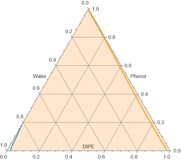
Experimental tie lines in dashed blue
Let us compute the RMSD
Tie line length
Final check
References
References
1. Zhang, F.; et al. Liquid–Liquid Equilibria for the Quaternary System: Diisopropyl Ether + n-Pentanol + Phenol + Water at 298.15 K. J. Chem. Eng. Data 2020, 65 (11), 5210. https://pubs.acs.org/doi/abs/10.1021/acs.jced.0c00539
2. Renon, H.; Prausnitz, J. M. Local Compositions in Thermodynamic Excess Functions for Liquid Mixtures. AIChE J. 1968, 14 (1), 135–144.
3. Abrams, D. S.; Prausnitz, J. M. Statistical Thermodynamics of Liquid Mixtures: A New Expression for the Excess Gibbs Energy of Partly or Completely Miscible Systems. AIChE J. 1975, 21 (1), 116–128.
4. Keller, H. B. Numerical Solution of Bifurcation and Nonlinear Eigenvalue Problems. In Applications of Bifurcation Theory; Rabinowitz, P. H., Ed.; Academic Press: New York, 1977; pp 359–384.
5. Sørensen, J. M.; Arlt, W. Liquid-Liquid Equilibrium Data Collection; DECHEMA Chemistry Data Series, Vol. V; DECHEMA: Frankfurt, 1979–1980.
CITE THIS NOTEBOOK
CITE THIS NOTEBOOK
Common tangent plane and arc-length continuation for computing LLE diagrams: DIPE + phenol + H2O
by Housam Binous
Wolfram Community, STAFF PICKS, August 3, 2026
https://community.wolfram.com/groups/-/m/t/3771895
by Housam Binous
Wolfram Community, STAFF PICKS, August 3, 2026
https://community.wolfram.com/groups/-/m/t/3771895