When a derivative can be written as a function of the independent variable only:
for example :
′
y
′′
y
′′′
y
etc
We call that a directly integrable equation
Example 1:
Example 1:
Find the general solution for the following directly integrable equation
dy
dx
2
x
That means
y∫6+4dx
2
x
y2+4x+c
3
x
c
So, is the general solution. It describes a family of functions that all satisfy the differential equation.
y2+4x+c
3
x
In[]:=
y'[x_]=6x^2+4
Out[]=
4+6
2
x
In[]:=
y[x_]=Integrate[y'[x],x,GeneratedParameters->C]
Out[]=
4x+2+
3
x
1
Example 2:
Example 2:
Find the particular solution for the following equation with condition
2
x
′
y
y(1)3
So we will need to get the by itself
′
y
′
y
-1
x
then
y-dx
1
2
x
so ,
y+c
1
x
c
And this is our general solution. Now we plug in the initial condition when
x1,y3
That means
c2
Thus, the particular solution is
y+2
1
x
In[]:=
Clear["Global`*"]
We can calculate the general solution as follows
In[]:=
y'[x]==-;
1
x^2
In[]:=
y[x]=Integrate[y'[x],x,GeneratedParameters->C]
Out[]=
1
x
1
and the we calculate the particular solution using the initial condition
In[]:=
SimplifyDSolvey'[x]==-,y[1]==3,y[x],x
1
x^2
Out[]=
y[x]2+
1
x
In[]:=
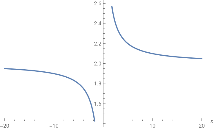
Plot[2+1/x,{x,-20,20},PlotRange->Automatic,AxesLabel->Automatic]
Out[]=
Example 3
Example 3
Find the particular solution for the following equation with condition
2
d
d
2
t
′
y
So the antiderivative is
dy
dt
c
1
the we use the initial condition
′
y
c0
So , sint , then
dy
dt
y-cost+
c
2
Now, we plug in our initial condition to our general solution and we get 2
y(0)1
c
2
Hence, the particular solution to our problem is
y-cost+2
In[]:=
Simplify[DSolve[{y''[t]==Cos[t],{y'[0]==0,y[0]==1}},y[t],t]]
Out[]=
{{y[t]2-Cos[t]}}
In[]:=
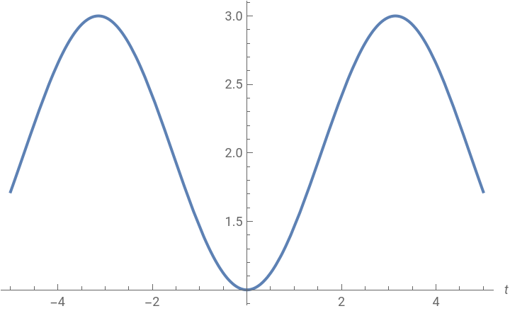
Plot[2-Cos[t],{t,-5,5},PlotRange->Automatic,AxesLabel->Automatic]
Out[]=