ABSTRACT (original article): This paper provides a pedagogical introduction to the classical nonlinear stability analysis of the plane Poiseuille and Couette flows. The whole procedure is kept as simple as possible by presenting all the logical steps involved in the application of the energy method and leading to the Euler-Lagrange equations. Then, the eigenvalue problems needed for the evaluation of the nonlinear energy threshold of the Reynolds number for stability are formulated for transverse modes and for longitudinal modes. Such formulations involve the streamfunction and, in the case of longitudinal modes, also the streamwise component of velocity. An accurate numerical solution of the eigenvalue problems, based on Galerkin’s method of weighted residuals with the test functions expressed in terms of Chebyshev polynomials, is discussed in details. The numerical codes developed for the software Mathematica 14 (© Wolfram Research, Inc.) are also presented. A critical analysis of the obtained results is finally proposed. CITATION (original article): Barletta, A., Mulone, G. Energy method and stability of shear flows: an elementary tutorial. Eur. Phys. J. Plus 139, 906 (2024). https://doi.org/10.1140/epjp/s13360-024-05720-z
Introduction
Introduction
This notebook is devoted to the hydrodynamic instability in shear flows taking place in a plane parallel channel. In particular, the study is focussed on the Poiseuille and Couette flows. The approach is based on the energy method. This means that an eigenvalue problem is developed starting from the determination of the maximum for a suitable functional of the velocity field that describes the perturbation of the base shear flow. The solution of the eigenvalue problem serves to provide the threshold in terms of the Reynolds number, , below which no instability may arise.
Re
In particular, the base flows considered here are expressed by the dimensionless velocity components along the Cartesian axes:where , COUETTE FLOW , POISEUILLE FLOWThe dimensionless spatial domain is .
x,y,z
U=f(z),V=0,W=0,
f(z)=z
f(z)=1-
2
z
x∈,y∈,z∈[-1,1]
More details regarding the problem formulation can be found in paper: https://doi.org/10.1140/epjp/s13360-024-05720-z
Joseph’s Method (L-modes eigenvalue problem)
Joseph’s Method (L-modes eigenvalue problem)
The solution method based on longitudinal modes, developed by D.D. Joseph, is illustrated with reference to the case of Poiseuille flow, , but it can be easily adapted to Couette flow by employing instead
U[z_]:=1-
2
z
U[z_]:=z
Definitions
Definitions
[ODE1]η''[z]-η[z]+REU'[z]φ[z]0[ODE2]φ''''[z]-2φ''[z]+φ[z]+REU'[z]η[z]0,[BC]φ[-1]0,φ'[-1]0,φ[1]0,φ'[1]0η[z]=ϕ[m,z];φ[z]=ψ[m,z]
2
α
α
2
2
α
4
α
α
2
∞
∑
m=0
b
m
∞
∑
m=0
a
m
A matrix eigenvalue problem is built by:
1) multiplying [ODE 1] by and integrating over z ∈ [-1,1]
2) multiplying [ODE 2] by and integrating over z ∈ [-1,1]
1) multiplying [ODE 1] by
ϕ[n,z]
2) multiplying [ODE 2] by
ψ[n,z]
In[]:=
NN=30;
In[]:=
U[z_]:=1-;
2
z
In[]:=
ϕ[n_,z_]:=(1-)ChebyshevT[n,z];
2
z
In[]:=
ψ[n_,z_]:=ChebyshevT[n,z];
2
(1-)
2
z
In[]:=
EchoTiming[Do[E0[n,m]=Integrate[ϕ[n,z]ϕ[m,z],{z,-1,1}],{n,0,NN},{m,0,NN}]];
⌚
29.2477
In[]:=
EchoTiming[Do[E2[n,m]=Integrate[ϕ[n,z]D[ϕ[m,z],{z,2}],{z,-1,1}],{n,0,NN},{m,0,NN}]];
⌚
18.424
In[]:=
EchoTiming[Do[EU0[n,m]=Integrate[ϕ[n,z]U'[z]ψ[m,z],{z,-1,1}],{n,0,NN},{m,0,NN}]];
⌚
31.438
In[]:=
EchoTiming[Do[A0[n,m]=Integrate[ψ[n,z]ψ[m,z],{z,-1,1}],{n,0,NN},{m,0,NN}]];
⌚
32.4341
In[]:=
EchoTiming[Do[A2[n,m]=Integrate[ψ[n,z]D[ψ[m,z],{z,2}],{z,-1,1}],{n,0,NN},{m,0,NN}]];
⌚
30.4253
In[]:=
EchoTiming[Do[A4[n,m]=Integrate[ψ[n,z]D[ψ[m,z],{z,4}],{z,-1,1}],{n,0,NN},{m,0,NN}]];
⌚
29.1377
In[]:=
EchoTiming[Do[AU0[n,m]=Integrate[ψ[n,z]U'[z]ϕ[m,z],{z,-1,1}],{n,0,NN},{m,0,NN}]];
⌚
31.1861
In[]:=
EE0[α_,M_]:=Table[E2[n,m]-E0[n,m],{n,0,M},{m,0,M}];
2
α
In[]:=
AA0[α_,M_]:=Table[A4[n,m]-2A2[n,m]+A0[n,m],{n,0,M},{m,0,M}];
2
α
4
α
In[]:=
AA[α_,M_]:=ArrayFlatten[BlockDiagonalMatrix[{EE0[α,M],AA0[α,M]}]];
In[]:=
BB[α_,M_]:=ArrayFlattenConstantArray[0,{M+1,M+1}],Table-EU0[n,m],{n,0,M},{m,0,M},Table-AU0[n,m],{n,0,M},{m,0,M},ConstantArray[0,{M+1,M+1}];
α
2
α
2
Generalized eigenvalue problem with c the eigenvalue and aa the eigenvector (vector of coefficients and)
AA[α,RE]aa = c BB[α] aa
The matrices AA and BB are 2(M + 1) × 2(M + 1)
The eigenvalue c is the Reynolds number denoted as RE
b
n
a
n
AA[α,RE]
·
·
The matrices AA and BB are 2(M + 1) × 2(M + 1)
The eigenvalue c is the Reynolds number denoted as RE
Calculations
Calculations
This is the array of the eigenvalues c for α = 2 and M = 30 ordered with increasing value of |c|
In[]:=
SortBy[With[{α=N[2,40],M=30},N[Chop[Eigenvalues[{AA[α,M],BB[α,M]}]],6]],N[Abs[Re[#]]]&]//MatrixForm
Out[]//MatrixForm=
-49.6203 |
49.6203 |
-61.7493 |
61.7493 |
-285.569 |
285.569 |
-342.711 |
342.711 |
-931.242 |
931.242 |
-1057.86 |
1057.86 |
-2207.40 |
2207.40 |
-2429.68 |
2429.68 |
-4333.47 |
4333.47 |
-4678.86 |
4678.86 |
-7529.93 |
7529.93 |
-8025.81 |
8025.81 |
-12017.3 |
12017.3 |
-12691.0 |
12691.0 |
-18016.6 |
18016.6 |
-18895.4 |
18895.4 |
-25751.6 |
25751.6 |
-26873.1 |
26873.1 |
-35691.9 |
35691.9 |
-37063.4 |
37063.4 |
-49921.2 |
49921.2 |
-51096.5 |
51096.5 |
-67328.6 |
67328.6 |
-74734.9 |
74734.9 |
-121233. |
121233. |
-126000. |
126000. |
-266810. |
266810. |
-336191. |
336191. |
-888889. |
888889. |
-1.80763× 6 10 |
1.80763× 6 10 |
∞ |
∞ |
The neutral stability curve data are obtained by detecting the lowest positive eigenvalue c for each given α
In[]:=
Do[With[{alpha=kk,M=20},aa=SortBy[Eigenvalues[{AA[alpha,M],BB[alpha,M]}],N[Abs[Re[#]]]&];alphaalpha=alpha;Print[{N[alphaalpha,4],Chop[Abs[aa[[1]]]]},","]],{kk,N[1/10,40],N[11+1/10,40],N[1/10,40]}]
{0.1000,582.9432788204334827660603514231716315804},
ShowListPlot,,Graphics[{PointSize[Large],Point[{2.043697448120342770592791089783399573089,49.60357834810872184681861010772548899220}]}]
Out[]=
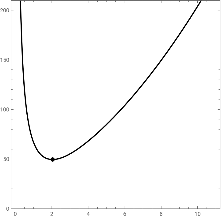
The minimum along the neutral stability curve is obtained by gradually restring the range of α
The sensitivity to the dimension of the matrix eigenvalue problem, 2(M + 1), is tested by considering different values of M
The sensitivity to the dimension of the matrix eigenvalue problem, 2(M + 1), is tested by considering different values of M
An accurate evaluation of the minimum along the neutral stability curve is obtained by generating and interpolating data in a narrow interval of α
The sensitivity to different settings of InterpolationOrder is also tested
The sensitivity to different settings of InterpolationOrder is also tested
Orr’s Method (T-modes eigenvalue problem)
Orr’s Method (T-modes eigenvalue problem)
Definitions
Definitions
Calculations
Calculations
This is the array of the eigenvalues c for α = 2 and M = 50 ordered with increasing value of |c|
The neutral stability curve data are obtained by detecting the lowest positive eigenvalue c for each given α
The minimum along the neutral stability curve is obtained by gradually restring the range of α
The sensitivity to the dimension of the matrix eigenvalue problem, M + 1, is tested by considering different values of M
The sensitivity to the dimension of the matrix eigenvalue problem, M + 1, is tested by considering different values of M
An accurate evaluation of the minimum along the neutral stability curve is obtained by generating and interpolating data in a narrow interval of α
The sensitivity to different settings of InterpolationOrder is also tested
The sensitivity to different settings of InterpolationOrder is also tested
CITE THIS NOTEBOOK
CITE THIS NOTEBOOK
Energy method and stability of shear flows: an elementary tutorial
by Antonio Barletta & Giuseppe Mulone
Wolfram Community, STAFF PICKS, December 10, 2025
https://community.wolfram.com/groups/-/m/t/3588903
by Antonio Barletta & Giuseppe Mulone
Wolfram Community, STAFF PICKS, December 10, 2025
https://community.wolfram.com/groups/-/m/t/3588903