Parking lots are often open, sunny spaces, making their roofs a fitting place to position solar panels. However, roofs are almost never perfectly rectangular. Additionally, solar panels must be meticulously positioned because photovoltaic solar cells generate the most electricity when sunlight strikes most directly. Even a few degrees of difference in measurements can cause significant losses over time. This optimization problem is complicated by the fact that the tilt angle and azimuth angle of the solar panels affects how many panels actually fit on the roof, and also how much power hits a single panel. In other words, an arrangement that maximizes the amount of tiles on the roof is not the same as an arrangement that maximizes the radiance that hits one panel. Another constraint is the fact that panels cast different lengths of shadows on each other at different distances and tilt angles. Additionally, celestial objects such as the sun itself ,which is constantly moving relative the Earth, and clouds, add variables to the power calculations. My project takes airport outlines from open street maps, uses mathematical formulas to optimize power based on the arrangement and tilt of solar panels, and visualizes optimal arrangements.
Introduction
Introduction
Renewable energy is quickly outpacing coal, and solar photovoltaics(PV) are experiencing an especially strong expansion globally. According to the International Energy Agency renewable electricity is projected to rise by 1050 Terawatt-hour (TWh) of which 600 TWh is expected to come from solar PV. In fact, 86 gigawatts of utility-scale electric generating capacity are supposed to be added the US power grid in 2026, where solar panels would make up 51% of that capacity addition. However, solar panels take up significant space, and thus require open, unshaded areas for higher efficiency. Many unused roofs, such as airport roofs provide this, so optimizing the placement and tilt of panels on these roofs is crucial. For this project, I aimed to optimize the tilt, azimuth, and packing method of solar panels across different latitudes based on the total solar irradiance hitting the panel.
Getting Polygons from Parking Lot Roofs
Getting Polygons from Parking Lot Roofs
Getting Data from Open Street Maps
Getting Data from Open Street Maps
Before starting solving the packing problem of putting solar panels in rows onto a polygon, I had to first get the polygon from an Open Street Maps dataset. In this case, I chose a random parking lot outline from the database to test. Since the coordinates from Open Street Maps are in latitude and longitude coordinates, they had to be converted to metric units first measured by the distance of each point to the the bottom left latitude of the polygon’s bounding box.
Imported data from open street maps, and used one of the roofs in the dataset to start with. Converted the latitude and longitude vertices into meters so that mapping panels onto the polygon would be easier later on.
Define a variable dataPoint comprised of all the data for this roof.
In[]:=
dataPoint=Association[dataset[[3]][[2]]];dataPoint//Dataset
Out[]=
Taking the shape from the data and setting it to a variable polygonOSM
In[]:=
polygonOSM=dataPoint["shape"];
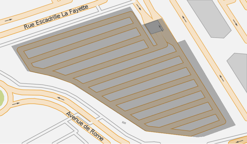
Visualizing using GeoGraphics to see how it looks on OSM
In[]:=
GeoGraphics[dataPoint["shape"]]
Out[]=
Visualizing just the polygon using Graphics
In[]:=
Graphics[dataPoint["shape"]]
Out[]=

Defining polygon coordinates
In[]:=
coordinates=GeoPosition/@polygonOSM[[1]]
Out[]=
{GeoPosition[{1.37701,43.6336}],GeoPosition[{1.37689,43.6338}],GeoPosition[{1.37563,43.6334}],GeoPosition[{1.3758,43.6331}],GeoPosition[{1.37602,43.6331}],GeoPosition[{1.37626,43.633}],GeoPosition[{1.3765,43.6328}],GeoPosition[{1.37656,43.6328}],GeoPosition[{1.37672,43.6327}],GeoPosition[{1.37673,43.6327}],GeoPosition[{1.37705,43.6325}],GeoPosition[{1.3776,43.6324}],GeoPosition[{1.37767,43.6324}],GeoPosition[{1.37801,43.6325}],GeoPosition[{1.37747,43.6334}],GeoPosition[{1.37739,43.6334}],GeoPosition[{1.37722,43.6337}],GeoPosition[{1.37701,43.6336}]}
Translate the polygon to {0,0}
In[]:=
bottomLeft=dataPoint["bbox"][[1]]geoPoints=(#-bottomLeft)&/@polygonOSM[[1]]
Out[]=
{1.37563,43.6324}
Out[]=
{{0.0013869,0.0011921},{0.0012627,0.0013861},{0.,0.0009664},{0.0001697,0.0007014},{0.0003923,0.0006553},{0.0006293,0.0005766},{0.000875,0.0004226},{0.000932,0.0003853},{0.0010887,0.0002827},{0.0011045,0.0002724},{0.0014198,0.000066},{0.0019772,0.},{0.002047,7.6×},{0.0023839,0.0001277},{0.0018435,0.0010349},{0.001763,0.0010043},{0.0015978,0.0012634},{0.0013869,0.0011921}}
-6
10
Converting to Metric System
Converting to Metric System
Latitude and longitude coordinates are based on a position on earth earth, which means the points I got in the last section were on a curved surface. However, because the dimensions of my solar panels are in meters, the Haversine formula was used to change the points from latitude and longitude to distance in meters from the bottom left of the bounding box. Finally, the entire polygon was translated back to the origin.
Convert to meters using Haversine formula
In[]:=
distanceMeters[latitude_,dlat_,dlon_]:=6371200*(2*ArcSin[Sqrt[(1-Cos[dlatDegree]+Cos[latitudeDegree]Cos[(latitude+dlat)Degree](1-Cos[dlonDegree]))/2.]])changeMeters[polygonCoordinates_,latitude_]:=Polygon[{distanceMeters[latitude,0,#[[1]]],distanceMeters[latitude,#[[2]],0]}&/@polygonCoordinates];
Use the distanceMeters function to change all of the vertices to distance in meters from the bottom left of the bounding box
In[]:=
metricPoints=changeMeters[geoPoints,bottomLeft[[1]]][[1]]
Out[]=
{{154.177,132.56},{140.37,154.132},{0.,107.462},{18.8648,77.9946},{43.6106,72.8683},{69.957,64.117},{97.2706,46.9924},{103.607,42.8447},{121.027,31.4358},{122.783,30.2905},{157.834,7.33916},{219.798,0.},{227.558,0.84383},{265.01,14.2002},{204.935,115.079},{195.986,111.677},{177.622,140.488},{154.177,132.56}}
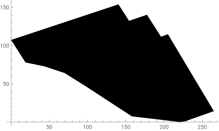
These converted points can be used to create a new polygon, which we can visualize to check the size of .
In[]:=
Graphics[Polygon[metricPoints],Axes->True]
Out[]=
This polygon is set to the variable polygon for further use later.
In[]:=
polygon=Polygon[metricPoints];
Packing Panels onto the Polygon
Packing Panels onto the Polygon
One of the most important things to consider when optimizing the arrangement solar panels is the amount of panels that can physically fit on the roof. This is determined by both the tilt of the panels and the azimuth angle of the panels. The optimal azimuth angle and tilt is different for each polygon based on their latitude and shape. Therefore, I had to create a function that would rotate the polygon based on an azimuth angle of the solar panels while keeping the rows of solar panels horizontal. This function also had to take the tilt of the panel and the distance between rows of panels (calculated later) to arrange the rows of solar panels on the roof.
First of all, the tilt of the solar panel has to be accounted for because a greater degree of tilt would mean the panels take up less space, and more importantly, would affect the distance between rows of panels. Thus, I made a function getPanelNums, that would take a polygon, a distance between rows, and the tilt of the panel, and return the number of panels that fit on the polygon. It is also good to note that the width used for calculating the arrangement will be which is the width of the area the panel takes up in birds eye view. Also, the length and width of the panel is set to 6 meters and 5 meters respectively, which is much bigger than a standard commercial solar panel, but I am using these measurements for this section to make the visualization easier to see. The function for distance between rows is added later.
Wp*Cos[tilt]
Set the length of the panel to 6 and the width of the panel to 5
In[]:=
Lp=6;Wp=5;distbwrows=5;
Find the line segments that cut across the polygon in rows and make an empty list, rowPanels, to store all the panels that fit on the line as the While loop runs.
In[]:=
getPanelsForRow[y_,W_,P_]:=Module[{intersect,xmin,xmax,currentX,rowPanels,rect},intersect=RegionIntersection[P,InfiniteLine[{{0,y},{1,y}}]];If[Head[intersect]===EmptyRegion,{},{xmin,xmax}=RegionBounds[intersect][[1]];currentX=xmin;rowPanels={};While[currentX+Lp<=xmax,rect=Rectangle[{currentX,y-W/2},{currentX+Lp,y+W/2}];If[RegionWithin[P,rect],AppendTo[rowPanels,rect];currentX+=Lp,currentX+=1]];rowPanels]]
The function listAllPanels returns a list of all the panels that fit inside of the polygon. Since the number of panels that fit on a polygon can change depending on the angle in which the rows are placed, the function also takes a rotation which will be optimized (as azimuth) in the final function
Calling getPanelsForRow for each y-value from half width to the maximum y-value of the RegionBounds of the polygon
An example output of this function can be visualized by setting values for tilt, distance, and rotation.
Visualizing polygons and panels using Graphics
Irradiance-related calculations
Irradiance-related calculations
Calculating Irradiance Per Panel
Calculating Irradiance Per Panel
When determining the optimal tilt angle and arrangement of solar panels, the ultimate goal is for the most power, or solar irradiance, to hit the panel. In order to optimize solar irradiance later, I created a function that takes the day, hour, tilt and azimuth of the panel, and latitude and returns an irradiance in Watts. These calculations are based on mathematical formulas from literature and websites which are specified throughout the code. Additionally, note that the final irradiance calculation accounts for both beam and diffuse irradiance, which is the radiant intensity from direct sunlight and light scattered by atmospheric components (such as clouds), respectively.
(Image from Hybrid Renewable Energy System for a Sustainable House-Power-Supply from the Journal of Advanced Research in Fluid Mechanics and Thermal Sciences)
For the demonstrations of each component of the instantaneous power function below, some example values were set for each of the inputs using the summer solstice as the example day, and the latitude of the center of the polygon for the latitude.
First, I defined the general variables. These are the variables used in both calculations for solar irradiance per panel, and distance between rows.
Solar declination angle is the angle between the equator and the line connecting the center of the Earth and the Sun. This value changes due to the Earth’s axial tilt and ranges from +23.45 degrees to -23.45 degrees depending on the time of year (Power Calculations, 2019).
Solar declination angle is the angle between the equator and the line connecting the center of the Earth and the Sun. This value changes due to the Earth’s axial tilt and ranges from +23.45 degrees to -23.45 degrees depending on the time of year (Power Calculations, 2019).
Hour angle is defined as the dihedral (intersection between two planes) angle between the observer’s meridian plane and the hour circle (Power Calculations, 2019).
Solar elevation angle between the line connecting the center of the sun to the observer, and the local horizontal planes (Power Calculations, 2019).
The solar zenith angle is defined as the angle between the Sun’s rays and the vertical line directly above the observer. This angle is complementary to the solar elevation angle (Power Calculations, 2019).
The solar azimuth angle is essentially the precise cardinal directions of the Sun (Yuehong et al., n.d.).
Then, I defined some variables specific to finding the solar irradiance of the panel.
Air mass ratio is the ratio between the distance of the observer to the sun, and the observer to the point right overhead (It can also be calculated as 1/Cos[β]) (Khatib & Wilfried Elmenreich, 2016).
Longitudinal incidence angle is the angle of the sun relative to the panel which depends on the azimuth and tilt of the panel (Duffie & Beckman, 2013).
Extraterrestrial flux is the rate that radiation from outside of the atmosphere reaches a certain area, in this case, the panel. (Power Calculations, 2019)
Optical depth is the amount of light from the sun that is scattered or absorbed by the atmosphere. (Power Calculations, 2019)
Finally we can calculate the direct sunlight (beam radiance), and sunlight scattered by atmospheric particles or reflected by clouds (diffuse radiance) (Khatib & Wilfried Elmenreich, 2016).
Beam irradiance
Diffuse irradiance
Lastly, we compute the sum of these two values, multiply by cosine of the incidence angle (considering Lamberts Cosine Law) , and then by the area of the panel.
The entire function is shown below with the example tilt of Pi/6.
Returning irradiance in Watts.
Adding Manipulate to graph how solar irradiance throughout the day changes with as latitude.
Another manipulate that shows how solar irradiance changes with tilt angle
Calculating Distance Between Rows
Calculating Distance Between Rows
When maximizing solar irradiance, it is also important to account for the shadow that one panel casts on another, and the best distance between rows that is obtained from that angle. A lot of the variables (solar declination angle, hour angle, solar elevation angle, solar zenith, and solar azimuth angle) used in the function for instantaneous solar irradiance are also used in my function for distance between rows. The two additional variables are shadow angle, and the actual calculation for distance between rows.
Angle of the shadow takes the azimuth and angle of the sun and is used for determining the optimal distance between rows. (Barbón et al., 2022)
Finding the best distance between the rows of solar panels. (Barbón et al., 2022)
The full function which returns a distance in meters (Barbón et al., 2022)
Optimizing Irradiance
Optimizing Irradiance
At this point all of the components that are required to optimize irradiance are prepared. The only thing left to do is to define a function for the irradiance during the vernal equinox that takes all of the variables, tilt, azimuth, latitude, and a polygon that will return the total power that hits the photovoltaic array throughout the whole day.
Calculate total irradiance for the vernal equinox throughout the day.
For the next function, I optimized the solar irradiance and found the tilt, azimuth, total panels, and total power for during the vernal equinox . For optimization, since I am testing this case with a latitude in the northern hemisphere and using the vernal equinox, I kept the tilt range between 10 and 40 degrees, which is a typical range for most panels, and the azimuth angle between 90 and 270 degrees.
Cycle through different tilt and azimuth angles to find the maximal daily power.
Visualizing Results
Visualizing Results
Although I was able to get the optimal measurements for tilt angle, azimuth angle, and the resulting total panels and total power, it is hard to see the trade off between number of panels that can be fit onto the polygon, and amount of power that hits each panel. To make this data more clear, I created a table to see the specific tilt and azimuth angles and their corresponding total panels and power.
Cycling through tilt from 10 degrees to 40 degrees in increments of 5 degrees, and cycling through azimuth angles between 90 degrees and 270 degrees in increments of 10 degrees.
Another way of visualizing this data is through a heat map.
X-axis is azimuth in radians, y-axis is tilt in radians, and power is represented by color.
Limitations and Conclusion
Limitations and Conclusion
In this project, I used various formulas to determine the optimal arrangement and positioning of solar panels on any polygon. In this case, I used the roof of an airport parking lot. I was able to generate visual representations of the packing algorithm used to fit all of the panels in the shape. By rotating the shape and changing the tilt of the solar panel, I was also able to find the perfect balance between solar irradiance per panel and amount of panels that actually fit on the roof.
However, there are some limitations of my optimization function one of which is the measurements I found depended on the position of the sun relative to the Earth, meaning it assumed optimal weather conditions throughout the year, and no shading by other objects, such as trees. Additionally, the optimization is based on the total irradiance during the vernal equinox only, and in order to change this to a wider range of days, I would improve my optimization function to run faster even while cycling through different azimuth and tilt angles. Nevertheless, my optimization algorithm was based on mathematical formulas from literature, and my results do align with typical solar panel placements, even though the time it takes the computer to get these results is not ideal.
However, there are some limitations of my optimization function one of which is the measurements I found depended on the position of the sun relative to the Earth, meaning it assumed optimal weather conditions throughout the year, and no shading by other objects, such as trees. Additionally, the optimization is based on the total irradiance during the vernal equinox only, and in order to change this to a wider range of days, I would improve my optimization function to run faster even while cycling through different azimuth and tilt angles. Nevertheless, my optimization algorithm was based on mathematical formulas from literature, and my results do align with typical solar panel placements, even though the time it takes the computer to get these results is not ideal.
Future Direction
Future Direction
In the future, I hope to expand this project to not only be able to pack solar panels on irregular polygons, but also other shapes with cutouts or rounded edges. Additionally, as I mentioned in limitations, I hope to maximize the annual irradiance, not for the vernal equinox. With that, I would also add the effect of weather conditions at the specific location throughout the year to get more precise calculations for annual irradiance.
References
References
Barbón, A., Ghodbane, M., Bayón, L., & Said, Z. (2022). A general algorithm for the optimization of photovoltaic modules layout on irregular rooftop shapes [Review of A general algorithm for the optimization of photovoltaic modules layout on irregular rooftop shapes]. Journal of Cleaner Production, 365, 132774. https://doi.org/10.1016/j.jclepro.2022.132774
Duffie, J. A., & Beckman, W. A. (2013). Solar engineering of thermal processes (4th ed.). Wiley. https://www.wiley.com/en-us/Solar+Engineering+of+Thermal+Processes%2C+4th+Edition-p-9780470873663
Khatib, T., & Wilfried Elmenreich. (2016). Modeling of Photovoltaic Systems Using MATLAB. John Wiley & Sons.https://catalogimages.wiley.com/images/db/pdf/9781119118107.excerpt.pdf
OpenStreetMap Wiki. (n.d.). Wiki.Openstreetmap.Org. Retrieved July 9, 2026, from https://wiki.openstreetmap.org/
Power Calculations, S. (2019). Mathematica Stack Exchange. Mathematica Stack Exchange. https://mathematica.stackexchange.com/questions/206602/solar-power-calculations
Wikipedia Contributors. (2019, August 7). Haversine formula. Wikipedia; Wikimedia Foundation. https://en.wikipedia.org/wiki/Haversine_formula
Yuehong, S., Jun, L., Jun, T., & Chong, S. (n.d.). Solar Azimuth Angle - an overview | ScienceDirect Topics [Review of Solar Azimuth Angle - an overview | ScienceDirect Topics]. Www.Sciencedirect.Com. Retrieved July 9, 2026, from https://www.sciencedirect.com/topics/engineering/solar-azimuth-angle
Acknowledgements
Acknowledgements
I would like to thank my mentor Piero Sanchez and all the TAs including Eric Archerman, Divya Thota, and Averyl Xu for helping me as I worked on my project! I would also like to express my gratitude to all of the directors Rory Foulger, Eryn Gillam, Megan Davis, and Cyrus Taylor, as well as Stephen Wolfram for helping me come up with this project idea.
CITE THIS NOTEBOOK
CITE THIS NOTEBOOK
Optimizing photovoltaic solar panel arrangement on irregularly shaped roofs
by Ellie Lee
Wolfram Community, STAFF PICKS, July 9, 2026
https://community.wolfram.com/groups/-/m/t/3751860
by Ellie Lee
Wolfram Community, STAFF PICKS, July 9, 2026
https://community.wolfram.com/groups/-/m/t/3751860