Wolfram Cloud Document

Code


Introduction

In this project, I’ve created a function I’ve called functionAutomaton that allows one to create a repeating pattern of cells containing functions, and then to connect the inputs to the functions to arbitrary other cells with functions in them, where the pattern in which the cells are connected also repeats. What I created this for to focus more on however was a specific case where the functions are binary boolean logic gates. I think this can be an interesting way to explore and visualize what certain kinds of arbitrary logic gate networks can do. The syntax I’ve use for specifying the gates is {{leftInput1, rightInput1}, gate1}, {leftInput2, rightInput2, gate2}...}. Inputs are specified by integers that say how many gates to the left and right the input comes from. Gates are specified by integers from 0-15 where the integer gives the Nth boolean function with 2 variables out of a possible 16 of them, as specified by the Wolfram Language BooleanFunction function.

Here’s code generating a table showing which integers correspond to some boolean functions:

In[]:=

#->FromDigits[Boole@BooleanTable[#[x,y],{x,y}],2]&/@{Nor,Xor,Nand,And,Implies,Or}

Out[]=

{Nor1,Xor6,Nand7,And8,Implies11,Or14}

And so given that, an input like this for example: {{{-1, 1}, 14}, {{1, 2}, 6}} would correspond to something like this:

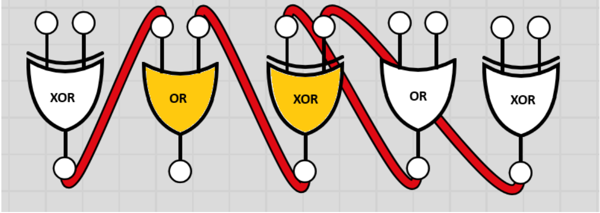
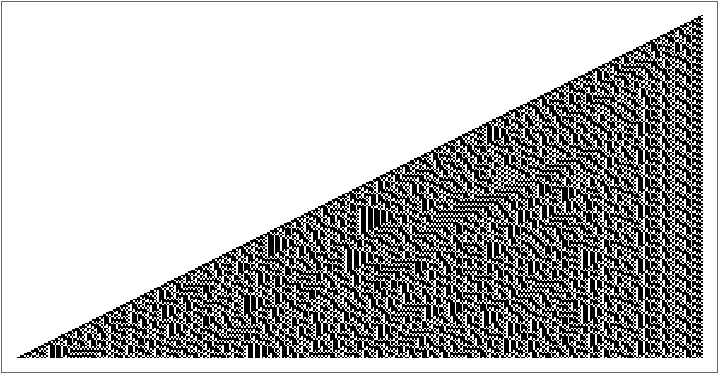
Where the highlighted gates are the specified ones, and the pattern of these two gates repeats forever to the left and right. Each OR gate takes its input from one gate to the left and one to the right, while each XOR gate takes input from one gate to the right and two gates to the right. The pattern of connections also repeats forever left and right, but here I’ve only showed the connections for the two highlighted gates to hopefully make it easier to see what’s going on. If one then turns on one of the OR gates, and lets the thing run for a few steps, one can get a pattern of on and off gates. Making the “on” gates black pixels and the “off” gates white, and then running the history down the page, one can get for this system of gates:

In[]:=

gA=booleanGateAutomaton[{0,1},{{{-1,1},14},{{1,2},6}},200];

In[]:=

ArrayPlot[gA[[All,;;Ceiling[Length[gA[[1]]]/2]]]]

Out[]=

Turing Completeness

The kinds of patterns this can make are certainly reminiscent of one dimensional cellular automata.

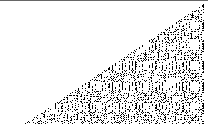
One can in fact set the system up to at least somewhat directly emulate a one dimensional cellular automaton. A 1D CA called rule 110 has been proven to be Turing complete, meaning that one can actually in principle get it to do any computation that any other computer could do, for instance. The computing that practical computers in everyday usage do is based on logic gates, and so one would think it shouldn’t be too surprising that one can do computations with this kind of system. Really one could in principle set up the logic gates to emulate a practical computer directly, and then use the infinite repeating array to network an infinite number of these computers together, say. Anyway, Aleksander Sabak and Discord user TARDIInsanity both helped me polish the syntax for this gate automaton system, and worked out rules that allow it to run rule 110. So here it is running on the rule they worked out together:

In[]:=

gA=booleanGateAutomaton[{1},{{{1,2},14},{{-1,2},6},{{-5,-2},2}},250];

In[]:=

ArrayPlot[gA[[All,Floor[Length[gA[[1]]]/6];;Ceiling[Length[gA[[1]]]/2]]]]

Out[]=

Gallery

Using only one gate I don’t think it’s possible to get it to do anything especially interesting. By experimenting I found however that with two gates it seemed easiest to get interesting non-repeating patterns when using two gates by using XOR gates mixed with some other gate. Through some exhaustive searches using XOR gates with certain other gates and certain short ranges for the connections, here is a gallery of a few findings, with rules and the patterns they generate starting again with having the first gate in the rule turned on with all the others off:

In[]:=

Multicolumn[Labeled[ArrayPlot[booleanGateAutomaton[{1,0},#,100],ImageSize->350],#]&/@Take[storedRules,{3,-1}],2]

Out[]=

{{{-1,1},1},{{1,2},6}}

{{{-1,1},7},{{-1,2},6}}

{{{-1,1},1},{{-1,2},6}}

{{{-1,1},7},{{1,2},6}}

{{{-1,0},1},{{1,2},6}}

{{{-1,1},11},{{-1,2},6}}

{{{-1,0},1},{{-1,2},6}}

{{{-1,1},11},{{1,2},6}}

{{{-1,1},14},{{-1,2},6}}

{{{-1,2},6},{{0,1},11}}

{{{-1,0},7},{{1,2},6}}

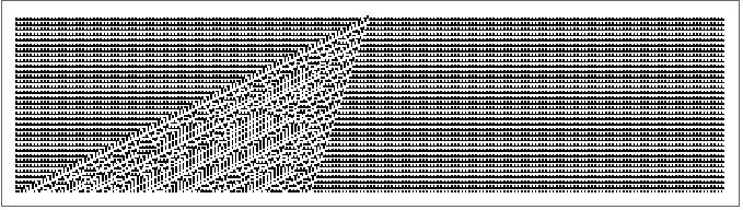
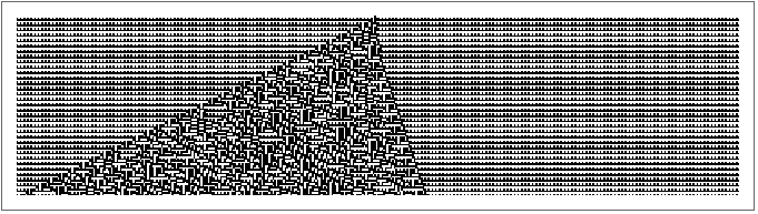
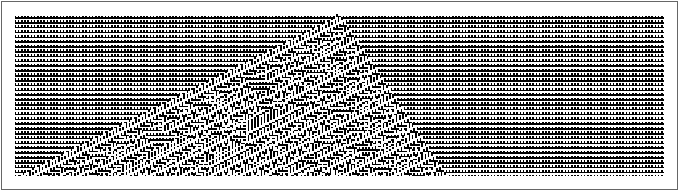
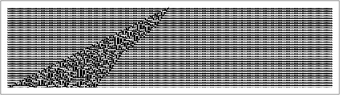
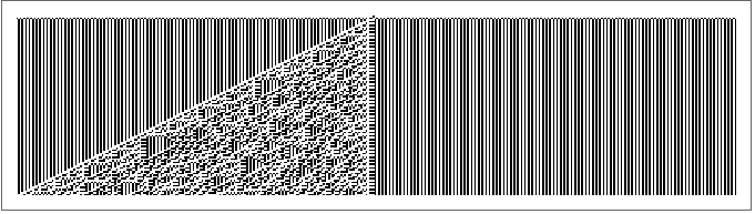
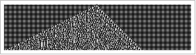
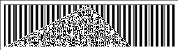
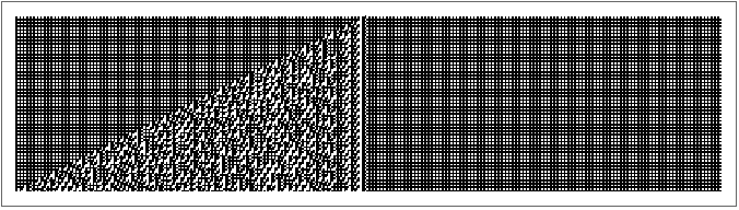
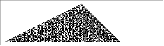
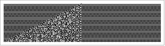
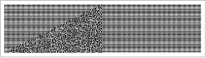
As for what “classes” these correspond to, as in cellular automaton classes, the most interesting ones I’ve found so far by searching are ones that look to me class 3, as in they look like they’ll generate complex but somewhat random behavior. The first rule above in the gallery, {{{-1, 1}, 1}, {{1, 2}, 6}}, looks to me like the most likely one that could possibly end up having persistent structures with different velocities meaning I feel like it could be class 4 in the end:

In[]:=

gA=booleanGateAutomaton[{1,0},{{{-1,1},1},{{1,2},6}},300];

In[]:=

ArrayPlot[gA[[All,;;Ceiling[Length[gA[[1]]]/2]]],ImageSize->Large]

Out[]=

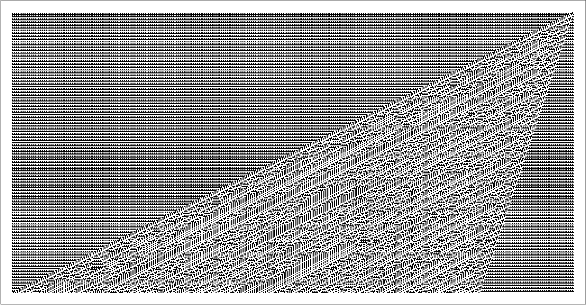
Rule 110 is known to be a class 4 cellular automaton however, so just due to that one knows it’s possible to have this system be class 4.

Conclusion

Simple 1D logic gate arrays are able to make interesting 1D cellular automaton like patterns, including emulating rule 110 which is known to be Turing complete and is thus a simple demonstration that this system can do any computation, in principle.

Interactive Demonstration

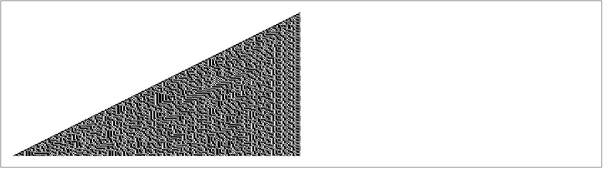
Finally, here is an interactive demonstration which includes the rules I’ve used above, and also allows the user to specify their own rules and initial conditions:

In[]:=

Manipulate[Quiet[ArrayPlot[booleanGateAutomaton[init,rule,steps],ImageSize->600],ArrayPlot::mat],{{rule,initRule,"Stored Rules"},storedRules,ControlType->PopupMenu},{{rule,initRule,"Custom Rule"},InputField[#,Expression]&},{{init,{1,0},"Init"},InputField[#,Expression]&},{{steps,200,"Steps"},1,250,1,Appearance->"Open"},SaveDefinitions->True]

Out[]=