The Wolfram Emerging Leaders Program: High School (WELP:HS) is a remote, semester-long program designed for exceptional graduates from the Wolfram High School Summer Research Program to continue to develop their skills. Students work in a small group over the course of a semester to do either a research-based project or a product development–based project under the guidance of expert mentors. Projects are centered around a topic at the intersection of the group’s interests.
Mentor: Safi Ahmed
Below-the-knee prosthetic limbs must simultaneously provide sufficient structural strength to support body weight and dynamic compliance to enable a natural, energy-efficient gait. This study analyzes prosthetic behavior through both structural mechanics and locomotion dynamics. First, a simplified below-knee prosthetic geometry is analyzed using finite element method (FEM) to estimate deformation, strain, and stress under a representative stance-phase load. Second, a spring-loaded inverted pendulum (SLIP) model captures the step-to-step locomotion dynamics of the leg at a system level. The SLIP model is then extended to a two-segment hip-knee system, where we derive how an effective leg stiffness depends on joint stiffness and knee angle, illustrating how overall leg compliance varies throughout a stride.
Introduction
Introduction
Below-the-Knee Prosthetic Limbs
Below-the-Knee Prosthetic Limbs
Below-the-knee prosthetic limbs must satisfy two difficult requirements: structural reliability under repeated high loads and support for stable, energy-efficient locomotion. During walking, load magnitude and direction vary throughout the gait cycle, thus it may experience substantially different stress patterns. A defensible analysis must therefore consider both material deformation under load and dynamic leg behavior during gait.
A Need to Analyze Solid Mechanics of Prosthetics and Walking Kinematics
A Need to Analyze Solid Mechanics of Prosthetics and Walking Kinematics
This essay employs computational tools to explore both sides of the problem. The first part treats the prosthetic like a solid object, where the FEM model identifies where a given geometry is most vulnerable to deformation, shown through displacement, strain, and stress across the leg. The second part shifts focus from materials to motion by modeling the step-to-step gait cycle using a simplified spring-leg system, then refining that model by adding a knee joint and examining how knee bending affects stiffness over time. We intend to establish a computational framework and interpretable stiffness relationships rather than produce clinical predictions.
Objectives
Objectives
The objectives of this computational essay were to:
1
.Construct a simple 3D prosthetic-leg geometry and compute displacement, strain, and stress fields under a representative axial stance-phase load using solid mechanics FEM analysis.
2
.Simulate a SLIP-based step cycle model and solve the governing differential equations, visualizing the progression apex → touchdown → stance → takeoff → apex.
3
.Extend the SLIP model to a two-segment hip-knee kinematic model, and connect knee/hip stiffness to an effective spring stiffness of the overall leg.
Solid Mechanics of an Imaginary Leg
Solid Mechanics of an Imaginary Leg
Creating the Limb
Creating the Limb
For this section, we create a below-the-knee prosthetic limb entirely out of steel. We simplify the prosthesis into a set of two coaxial cylinders, as shown in the figure below. The geometry is intentionally idealized to isolate the mechanical response of the prosthesis while excluding joint-complexity. This allows us to examine first-order mechanical behavior (load paths and stress concentration trends) without computationally demanding features such as sockets or anisotropic composite layups.
Figure:Simplificationofabelow-the-kneeprosthesisintoacompositecylinder |
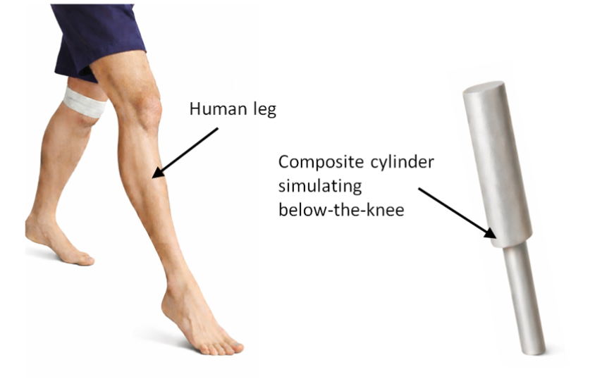
The thicker section of the composite cylinder represents the upper shank, while the thinner section represents the lower shank. This simplified geometry serves as the domain for the FEM analysis, where we compute displacement, strain components, and stress measures such as von Mises stress to examine the mechanical response of the model.
The first step in this process is to create a 3-D mesh of the prosthetic. To achieve this, we start by importing the FEM package of Wolfram:
Import the FEM package of Wolfram and set History Length to zero to avoid caching issues:
In[]:=
Needs["NDSolve`FEM`"]$HistoryLength=0;
Define geometric dimensions of the composite limb:
In[]:=
h1=.4;h2=0.6;rThin=0.05;rThick=0.075;
Construct upper and lower cylindrical segments:
In[]:=
thinCylinder=Cylinder[{{0,0,0},{0,0,h1}},rThin];thickCylinder=Cylinder[{{0,0,h1},{0,0,h1+h2}},rThick];
Combine the cylindrical segments and generate the mesh Ω:
In[]:=
legRegion=RegionUnion[thinCylinder,thickCylinder];Ω=ToElementMesh[DiscretizeRegion[legRegion,MeshRefinementFunction->(RegionMeasure[#1]>0.002&),MeshQualityGoal->1]];
The resulting element mesh discretizes the simplified geometry into finite elements suitable for stress and strain computation. A mesh refinement condition is applied to ensure adequate resolution in regions where geometric transitions may influence local stress distributions.
Visualize the generated mesh:
In[]:=
Ω["Wireframe"]
Out[]=
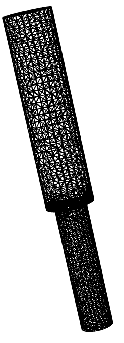
The wireframe view confirms the successful generation of the finite element mesh over the entire domain Ω.
Deformation Under Representative Stance-Phase Loading
Deformation Under Representative Stance-Phase Loading
We first analyze the leg under a representative stance-phase load, where the body weight is primarily transmitted axially through the prosthetic. We use Wolfram’s FEM tools to analyze the solid mechanics of the constructed model by defining a corresponding PDE formulation.
We first define the displacement field variables u, v, and w, representing motion in the x, y, and z directions.
Define the displacement field variables:
In[]:=
vars={{u[x,y,z],v[x,y,z],w[x,y,z]},{x,y,z}};
Then, we define the parameters for the material used. As we decided to use steel, we define the object’s parameters as seen below.
Specify material parameters for steel:
In[]:=
pars=<|"YoungModulus"->210*10^9,"PoissonRatio"->0.3,"MassDensity"->7850,"ThermalExpansion"->8.6*10^-6|>;
We apply a 686 N load in the negative z-direction at the top surface (z = h1 + h2), corresponding to the gravitational force of a 70 kg individual (70 × 9.81 m/s²), and impose a fixed constraint at the base (z = 0) to represent ground support.
Define boundary load and fixed constraint:
In[]:=
ΓForce=SolidBoundaryLoadValue[z==0,vars,pars,<|"Force"->{0,0,Quantity[686,"Newtons"]}|>];ΓWall=SolidFixedCondition[z==h1+h2,vars,pars];
Next, we define the solid mechanics PDE using the built-in SolidMechanicsPDEComponent under the imposed boundary conditions. This component internally formulates the displacement-based equilibrium equations using the specified material parameters and boundary conditions.
Construct the solid mechanics PDE operator:
In[]:=
op=SolidMechanicsPDEComponent[vars,pars];MatrixForm[op]
Out[]//MatrixForm=
∇ {x,y,z} 11 10 10 10 10 10 ∇ {x,y,z} ∇ {x,y,z} 11 10 10 10 ∇ {x,y,z} ∇ {x,y,z} 11 10 10 10 ∇ {x,y,z} |
∇ {x,y,z} 10 10 11 10 10 10 ∇ {x,y,z} ∇ {x,y,z} 10 10 11 10 ∇ {x,y,z} ∇ {x,y,z} 11 10 10 10 ∇ {x,y,z} |
∇ {x,y,z} 10 10 10 10 11 10 ∇ {x,y,z} ∇ {x,y,z} 10 10 11 10 ∇ {x,y,z} ∇ {x,y,z} 10 10 11 10 ∇ {x,y,z} |
We solve the resulting boundary-value problem using NDSolveValue to obtain the displacement field {u, v, w} over the domain Ω.
Solve the boundary-value problem for the displacement field:
In[]:=
legDisplacement=NDSolveValue[{op==ΓForce,ΓWall},{u[x,y,z],v[x,y,z],w[x,y,z]},{x,y,z}∈Ω];
The solver returns three interpolating functions corresponding to the displacement components u, v, and w, reflecting the vector-valued nature of the three-dimensional elasticity problem.
Visualizing the Deformation
Visualizing the Deformation
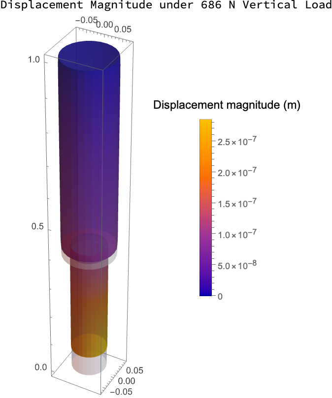
To visualize the displacements calculated above, we use the plot below. The colors represent the deformed configuration, with the legend on the right mapping displacement values (in meters) to the corresponding colors. The deformation is not shown to scale; the displacement has been deliberately exaggerated to make it easier to verify that all forces and displacements act in the correct directions. The color distribution and the legend on the right are what carry the physical meaning.
Visualize the displacement field using a 3D vector plot:
LabeledVectorDisplacementPlot3DlegDisplacement,{x,y,z}∈Ω,,"Displacement Magnitude under 686 N Vertical Load",Top
Out[]=
To further illustrate the deformation, we visualize both the undeformed and deformed configurations in exaggerated form.
Compute the deformed finite element mesh:
Overlay undeformed and deformed mesh configurations:
The deformation pattern reflects bending under vertical loading, with displacement increasing along the length from the fixed base toward the loaded top surface.
Calculating the Strain on the Leg
Calculating the Strain on the Leg
To quantify the deformation more precisely, we compute the strain tensor derived from the displacement field.
Compute the strain tensor from the displacement field:
Calculating the Stresses in the Leg
Calculating the Stresses in the Leg
Compute the Stress Tensor
Compute the Stress Tensor
Using the strain tensor computed above, we now compute the corresponding stress tensor based on the defined material properties of steel.
Compute the stress tensor from the strain field:
von Mises Stress
von Mises Stress
To assess whether the prosthetic would approach yielding under the applied load, we compute the von Mises equivalent stress. Unlike individual normal stress components, the von Mises stress condenses the full three-dimensional stress state into a single scalar measure suitable for comparison with material strength.
Compute the von Mises equivalent stress field and evaluate its minimum and maximum values:
Visualizing von Mises Stress:
The nearly uniform von Mises distribution is consistent with a predominantly uniaxial compressive stress state under symmetric axial loading.
Having verified that the structure remains within the elastic regime under representative stance loading, we now examine how effective stiffness influences walking dynamics using a reduced-order SLIP model.
The Cycle of a Step
The Cycle of a Step
Using the Spring-Loaded Inverted Pendulum (SLIP) model, each step of a prosthetic gait can be decomposed into distinct phases defined by key events: apex (maximum center-of-mass height), touchdown (initial ground contact), stance, and take-off (loss of ground contact). This reduced-order representation captures how the leg compresses, stores elastic energy, and re-extends during locomotion (Bhounsule, 2021).
Figures (a) and (b) below illustrate how a two-link hip-knee system can be configured through coordinated joint motion to reproduce the effective leg-length and stiffness behavior of a SLIP model during a gait cycle.
Here, apex denotes the instant of maximum center-of-mass height, touchdown marks initial ground contact, and take-off corresponds to loss of contact. In the SLIP abstraction, the leg is modeled as a massless spring of stiffness k supporting a lumped body mass. This simplification isolates the dominant axial dynamics of locomotion while neglecting higher-order joint complexity.
Mathematical Modeling
Mathematical Modeling
We define the physical and geometric parameters governing the model, including the body mass m, gravitational acceleration g, leg spring stiffness k, uncompressed leg length l₀, and the apex leg angle θ measured from the vertical. For conceptual clarity, we use representative parameter values that capture the qualitative behavior of the SLIP model rather than calibrating to a specific subject.
Set SLIP model parameters:
Solving for the Different Phases of a Step
Solving for the Different Phases of a Step
At the Apex
At the Apex
The step cycle is initialized at the apex, defined as the highest point of the mass trajectory during flight. At this configuration, the vertical velocity is zero by definition. We set the horizontal position to zero without loss of generality and choose the vertical position to exceed the geometric touchdown height l₀ cos(θ), ensuring that the motion begins in flight prior to ground contact.
Specify initial apex position for the SLIP step cycle:
A nonzero horizontal velocity initiates forward progression of the mass. By definition of the apex, the vertical velocity is zero at this instant. During the subsequent flight phase, motion is governed solely by gravitational acceleration.
Specify initial apex velocities for the SLIP step cycle:
During the Apex-Stance Phase
The interval between apex and touchdown constitutes the flight phase. During this phase, the mass follows ballistic motion under constant gravitational acceleration, with no spring interaction until ground contact.
In this phase, the leg’s motion can be described by the following initial value problem (IVP), with the horizontal displacement given by:
Similarly, the vertical displacement is given by:
The flight-phase initial value problem is solved until the geometric touchdown condition is satisfied. This occurs when the vertical coordinate reaches y(t) = l₀ cos(θ), corresponding to contact between the mass and the ground at the prescribed leg angle.
Solve the flight-phase initial value problem from apex to touchdown:
The event-driven termination defines the transition between continuous flight dynamics and the subsequent stance phase . The state at touchdown, obtained from the interpolating functions, provides the initial conditions for the next segment of the step cycle.
At the Touch Down
At the Touch Down
At touchdown, the state of the system must be extracted to initialize the stance phase dynamics. The touchdown time and corresponding position and velocity are obtained from the flight-phase solution.
Extract touchdown time from the flight-phase solution:
The extracted touchdown time defines the transition instant between flight and stance.
Evaluate touchdown position from the flight-phase solution:
Evaluate touchdown velocity from the flight-phase solution:
These values define the complete state of the mass at ground contact and serve as the initial conditions for the stance-phase model.
Compute ground contact point from touchdown geometry:
The ground contact point is determined from the touchdown geometry and remains fixed during the stance phase.
During the Stance Phase
During the Stance Phase
During the stance phase, the mass interacts with the ground through the spring anchored at the touchdown point. The governing equations incorporate leg compression forces along the instantaneous leg direction together with gravitational acceleration.
The horizontal displacement is given by:
The vertical displacement is given by:
The initial conditions for this phase are taken directly from the touchdown state computed during flight. This enforces continuity of position and velocity across the phase transition.
Solve the stance-phase initial value problem from touchdown to takeoff:
Values At Take Off
Values At Take Off
At takeoff, the state of the system is extracted to initialize the subsequent flight phase. The takeoff time and corresponding position and velocity are obtained from the stance-phase solution.
Extract takeoff time from the stance-phase solution:
The extracted takeoff time marks the completion of the stance phase and the transition back to flight.
Evaluate takeoff position from the stance-phase solution:
Evaluate takeoff velocity from the stance-phase solution:
These values define the complete state of the mass at takeoff and serve as the initial conditions for the next flight segment of the step cycle.
During the Stance to Apex phase
During the Stance to Apex phase
Following takeoff, the system re-enters the flight phase. The mass moves ballistically under gravitational acceleration, with initial conditions determined by the takeoff state. This phase continues until the vertical velocity again becomes zero, marking the next apex.
Solve the flight-phase initial value problem from takeoff to apex:
The flight-phase initial value problem is terminated when y’(t) = 0, corresponding to the highest point of the trajectory. This defines the completion of one full step cycle.
Together, the apex, touchdown, takeoff, and subsequent apex events define a complete step cycle within the SLIP model.
Visualizing the Step
Visualizing the Step
Now that we’ve solved for the three phases of the step, we can plot the x and y coordinates of the leg over time.
Visualize the complete step trajectory across flight and stance phases:
The x–y trajectory over one step illustrates the piecewise dynamics of the SLIP model. The flight segments correspond to ballistic motion under gravity, while the stance segment captures spring compression followed by re-extension. The minimum height occurs during stance, at the point of maximum leg compression prior to upward re-acceleration toward the next apex.
Construct cumulative event times for the full step cycle:
These event times define a unified timeline across phases, and enable the construction of the animation of the step cycle.
The animation illustrates the evolution of the center of mass and leg configuration over one step, and makes the phase transitions and spring compression visually explicit.
The same step is shown in a body-fixed frame below. We recenter the frame in the horizontal direction so that the center of mass remains fixed. This allows the leg angle and spring compression to be visualized more clearly.
In this view, the touchdown angle is clearly visible, followed by progressive leg compression during stance as the hip lowers to its minimum height, and subsequent re-extension until takeoff when the leg reaches its rest length again. Together, the inertial and body-fixed views complete the simulation of one SLIP step cycle, linking the phase-wise differential equation solutions to a continuous apex → touchdown → stance → takeoff → apex progression.
Translating a Single Limb to Implement a Knee
Translating a Single Limb to Implement a Knee
The two-segment representation is constructed so that the hip and foot positions coincide with those of the original SLIP virtual leg, preserving endpoint geometry while introducing joint-level structure. The position of the foot relative to the hip can be expressed by the vector p, where:
The endpoint position of the foot is obtained through forward kinematics of the two-link chain. Expressing the foot coordinates in terms of the link lengths and joint angles establishes a direct geometric mapping between joint configuration and overall leg length. This will form the basis for relating joint stiffness to an effective leg stiffness which is presented in the subsequent sections.
The SLIP motion was previously computed in separate temporal phases. To embed this motion within the two-segment representation, we reconstruct the global hip position as a single time-dependent function.
Define global hip position hipPos[t] from phase-specific solutions:
This provides a continuous global representation of the hip trajectory across all motion phases.
With the hip trajectory defined, the foot position is constructed piecewise in time. During flight phases, the foot is positioned relative to the hip by adding or subtracting a leg vector of fixed length l₀ oriented at angle θ, expressed as l₀{sin θ, −cos θ}. During stance, the foot remains fixed at the ground contact point (xC, 0).
Define global foot position footPos[t] from hip position and phase logic:
With both hip and foot positions defined in global coordinates, the relative leg vector can now be obtained by subtraction. The relative leg vector pVec is defined as the displacement from the hip to the foot.
Define relative foot position vector pVec[t] and its components:
The vector pVec[t] represents the instantaneous leg configuration in Cartesian coordinates. Its magnitude corresponds to the effective leg length and will be used to relate joint-level stiffness to overall leg stiffness.
Before proceeding, we verify consistency of the reconstructed hip, foot, and relative leg positions at the initial time.
Evaluate hip, foot, and relative leg positions at t = 0:
The relative vector pVec[0] equals footPos[0] − hipPos[0], confirming that the geometric reconstruction is internally consistent.
We now assign physical segment lengths to the two-link representation.
Define segment lengths l₁ and l₂:
These lengths are chosen such that l₁ + l₂ = l₀, ensuring that the fully extended two-segment leg matches the original SLIP virtual leg length.
The instantaneous leg length is obtained from the Cartesian components of the relative leg vector.
Define scalar leg length legL[t] as the magnitude of pVec[t]:
This scalar length represents the effective leg length and provides the geometric quantity through which joint-level stiffness will be related to overall leg compliance.
The joint angles θ₁[t] and θ₂[t] are recovered from the geometric configuration of the two-segment leg. The hip angle θ₁[t] is expressed in terms of the Cartesian leg vector and the knee angle θ₂[t], while θ₂[t] itself is determined from the instantaneous leg length using the law of cosines.
Define hip angle θ₁[t] from leg geometry and θ₂[t]:
Define knee angle θ₂[t] from leg length using the law of cosines:
The cosine argument is clipped to the valid domain [−1, 1] of ArcCos to prevent small floating-point errors from producing complex values.
Although θ₁[t] appears before θ₂[t] in the notebook, both are evaluated consistently once the geometric relations are fully defined.
To confirm the behavior of the recovered knee angle, we evaluate θ₂[t] at representative time points.
Evaluate θ₂[t] at representative time points:
The values confirm that θ₂[t] varies smoothly and remains within the expected geometric range during the motion.
With the joint angles and endpoint positions defined, the knee position can be reconstructed geometrically.
Define knee position kneePos[t] from two-link geometry:
The knee position is obtained by reconstructing the triangle formed by the hip, knee, and foot. Starting from the hip, we move a distance h along the line connecting the hip and the foot, and then offset perpendicularly to satisfy the fixed segment lengths l₁ and l₂. The chosen sign selects the backward-bending knee configuration.
Animating the Leg with a Knee
Animating the Leg with a Knee
To visualize, we can again animate the walking leg, this time with a knee joint.
The animation confirms that the reconstructed hip–knee–foot configuration remains geometrically consistent throughout the motion. The two-link representation reproduces the SLIP trajectory while introducing joint-level structure without altering the overall endpoint kinematics.
Deriving the Spring Stiffness Coefficient for the Knee
Deriving the Spring Stiffness Coefficient for the Knee
In the SLIP model, the leg is represented as a single axial spring with stiffness k. To realize this behavior using a two-segment leg with hip and knee joints, we derive how small joint rotations map to changes in the virtual leg length. This allows us to relate the axial stiffness of the virtual leg to equivalent torsional stiffnesses at the hip and knee joints.
Consider the relative foot position vector p as defined above. Differentiating with respect to time yields:
The matrix of partial derivatives is denoted by J, the Jacobian of the two-link system. It maps joint angular velocities to the linear velocity of the foot.
The Jacobian J[t] is defined by the partial derivatives of the foot position with respect to the joint angles.
Define the Jacobian matrix J[t] = ∂p/∂θ:
For small joint variations, the differential relationship becomes:
This linearized mapping provides the geometric link needed to relate joint torques to effective axial stiffness of the virtual leg.
The unit vector u along the virtual leg, pointing from the hip to the foot, is defined as
Define unit leg direction u[t] = p/‖p‖:
To relate joint motion to axial stiffness, we need the change in the virtual leg length L rather than the full two-dimensional displacement δp. Since L is the magnitude of p, small changes in length are obtained by projecting δp onto the unit leg direction u. This gives:
where the 1×2 row vector uᵀ multiplied by the 2×1 displacement vector δp produces a 1×1 scalar. This scalar represents the axial extension or compression of the leg.
Realizing that δp = Jδθ, we have:
Since J is a 2×2 matrix and uᵀ is a 1×2 row vector, their product uᵀ J is a 1×2 row vector. Denoting its components by a₁ and a₂ gives:
Plugging back into the expression for δL, we get:
Thus the coefficients a₁ and a₂ quantify how small rotations at the hip and knee contribute to changes in the virtual leg length.
The coefficients a₁ and a₂ are now evaluated explicitly as functions of time.
Define sensitivity vector [a₁ a₂] = uᵀ J:
Evaluate a₁[t] and a₂[t] at representative time points:
These values reflect how the leg posture determines which joint controls the effective leg length. Near t = t₁, the leg is relatively extended, so rotating either the hip or knee tends to move the foot outward along the leg direction. Both a₁ and a₂ are therefore positive, with the hip contributing more strongly.
By mid-stance, the geometry changes: hip rotation mostly swings the leg sideways rather than lengthening it, so a₁ becomes small. In contrast, knee rotation now directly alters the separation between hip and foot, and the negative value of a₂ indicates that increasing knee flexion shortens the virtual leg.
Utilizing the principle of virtual work
Utilizing the principle of virtual work
We begin with the geometric relationship already obtained for the two-segment leg:
This expression shows that small changes in leg length arise from joint rotations, with a₁ and a₂ quantifying the sensitivity of the overall leg length to hip and knee rotations, respectively. We first isolate the hip contribution by holding the knee fixed (δθ₂ = 0). This gives us:
This expression shows that small changes in leg length arise from joint rotations, with a₁ and a₂ quantifying the sensitivity of the overall leg length to hip and knee rotations, respectively. We first isolate the hip contribution by holding the knee fixed (δθ₂ = 0). This gives us:
From earlier, we deduced that F is the axial force that compresses the virtual leg, acting along the leg direction and producing the leg-length change δL. If the leg shortens by a small amount of δL under this force, the work done by the force can be written as:
δW = F δL
The principle of virtual work states that different descriptions of the same small physical motion must yield the same work. Therefore, the two expressions for δW can be equated.
Because the same virtual rotation δθ₁ appears on both sides, it can be factored out, yielding:
Each joint is modeled as a linear torsional spring and therefore resists rotation with a torsional stiffness. By definition:
Equating these with the torque expressions above yields:
Solving for the joint rotations, we get:
Or
The computed values show that the required knee torsional stiffness varies between touchdown and mid-stance. As the geometric influence of the knee on leg shortening changes, the torsional stiffness needed to reproduce the same axial stiffness k also changes.
Plotting the Torsional Stiffness Coefficient for the Knee
Plotting the Torsional Stiffness Coefficient for the Knee
Plot the required knee torsional stiffness kθ,knee[t] over one gait cycle (apex → apex):
Immediately after touchdown, the curve drops sharply. This indicates that a smaller torsional stiffness at the knee is sufficient to maintain the same axial leg stiffness. In this configuration, knee rotation becomes highly effective at producing axial shortening of the virtual leg.
As stance progresses toward mid-stance, the stiffness rises again. Here, knee rotation becomes less effective at altering the virtual leg length, so a larger torsional stiffness is required to preserve the same apparent axial stiffness k.
The abrupt transitions near phase boundaries arise from the piecewise SLIP reconstruction, which introduces geometric discontinuities.
The stiffness curve clearly varies over time, but it does not immediately reveal why it varies. From the derived relationship,
Plot the geometric sensitivity a₂(t) over one gait cycle:
The coefficient a₂(t) represents how strongly a small knee rotation changes the virtual leg length at each instant. It is the axial projection of knee-induced foot motion onto the hip–foot line.
Reading this curve from left to right, a₂ is initially positive and nearly constant near apex. This indicates that knee rotation produces a modest and consistent change in leg length.
Immediately after touchdown, a₂ decreases rapidly and becomes negative. The sign change indicates that the direction of axial motion induced by knee rotation reverses: increasing knee flexion now shortens the leg rather than lengthening it. The magnitude |a₂| becomes large in this region, meaning knee rotation is highly effective at producing axial shortening.
As stance progresses toward mid-stance, |a₂| gradually decreases again as the geometric alignment between knee rotation and the hip–foot axis changes. Near the phase boundary, a₂ returns to its initial positive value.
Thus, the variation in required knee stiffness over the gait cycle is fundamentally geometric: it reflects how effectively knee rotation contributes to axial shortening of the virtual leg at each instant.
This analysis shows that a constant axial stiffness k does not imply constant joint stiffness. Even with fixed hip stiffness, the required knee stiffness varies substantially over the gait cycle due purely to geometry. In a physical prosthetic system, this suggests that a passive linear torsional spring would only match the desired axial behavior at one configuration. Achieving consistent axial behavior across stance would require either configuration-dependent stiffness or an adaptive mechanism.
Conclusion
Conclusion
This computational essay examined a simplified below-the-knee prosthetic model from two complementary perspectives: structural deformation under representative stance-phase loading and reduced-order modeling of gait dynamics over a stride. The solid mechanics analysis quantified displacement, strain, and stress in a fixed limb geometry subjected to a prescribed stance-phase load, establishing how the structure responds under realistic loading conditions.
The gait modeling section began with a SLIP-based representation of leg dynamics, with motion computed phase by phase and then assembled over a full stride. Extending this model to a two-segment hip–knee representation allowed the virtual leg length to be expressed in terms of joint rotations. Using a geometric mapping and virtual work, the effective axial stiffness was related to joint torsional stiffness, revealing that the apparent leg stiffness depends strongly on configuration rather than being a fixed material property.
Taken together, the structural and dynamic analyses demonstrate how mechanical behavior is shaped by geometry at different modeling scales. In the structural model, the fixed limb geometry governs how stance-phase forces generate displacement and stress within the material. In the dynamic model, the same geometric configuration determines how joint rotations project onto axial leg shortening, thereby reshaping the apparent stiffness of the virtual leg. Although the two models operate at different levels of abstraction, both reveal that load response and effective stiffness emerge from configuration rather than from material parameters alone.
The study demonstrates how simplified but structured models can reveal the role of geometry in governing stress distribution and effective stiffness. Even at reduced levels of abstraction, careful mathematical formulation makes it possible to trace how configuration shapes mechanical response.
Acknowledgements
Acknowledgements
We would like to thank our mentor, Safi Ahmed, for his steady guidance throughout this project. His support in shaping our approach, troubleshooting the code, and explaining the physics behind our models made this work possible and helped us turn a complex idea into clear, meaningful results. We also extend our sincere gratitude to Dr. Hamza Asif at NUST for his guidance on the theoretical foundations and derivations. Finally, we thank Rory, Eryn, and the Wolfram Education team for providing an invaluable learning experience throughout the Wolfram Emerging Leaders Program.
References
References
◼
Bhounsule, P. (2021, February 25). Legged robotics 12b: Spring-loaded inverted pendulum model (Spring 2021) [Video]. YouTube. https://www.youtube.com/watch?v=qI_94iU1S0c
◼
Campanelli, L. (2023). A simple model of human walking. Journal of Medical Science, 92(1), 817. https://doi.org/10.20883/medical.e817
◼
Karim, A. A. (2012). Procedural locomotion of multi-legged characters in complex dynamic environments: Real-time applications (Doctoral dissertation, Université Claude Bernard Lyon 1). https://tel.archives-ouvertes.fr/tel-01165192
◼
Khan Academy. (2011, September 17). Differential equation introduction: First-order differential equations [Video]. YouTube. https://www.youtube.com/watch?v=6o7b9yyhH7k
◼
Schwind, W. J., & Koditschek, D. E. (2000). Approximating the stance map of a 2-DOF monoped runner. Journal of Nonlinear Science, 10, OF1–OF36. https://doi.org/10.1007/s003320010001
◼
Wang, L.-I. (2008). The kinetics and stiffness characteristics of the lower extremity in older adults during vertical jumping. Journal of Sports Science & Medicine, 7(3), 379–386. https://pmc.ncbi.nlm.nih.gov/articles/PMC3761894/
CITE THIS NOTEBOOK
CITE THIS NOTEBOOK
Modeling below-the-knee prosthetics using FEM and SLIP dynamics
by Arnay Garhyan, Eunchan Hwang, and Bryan Chen
Wolfram Community, STAFF PICKS, February 17, 2026
https://community.wolfram.com/groups/-/m/t/3641221
by Arnay Garhyan, Eunchan Hwang, and Bryan Chen
Wolfram Community, STAFF PICKS, February 17, 2026
https://community.wolfram.com/groups/-/m/t/3641221