Option pricing
Option pricing
This notebook continues the evaluation of the Schwab API with option price data. October calls and puts are examined. Prices are calculated using the implied volatility measure given by Schwab and the implied volatility calculation from the Black-Scholes call formula. The results suggest that you should do your own price calculations from the data. The volatility offered by the API appears not to be calculated from the data. The FinancialDerivative[] models seem to work well with a volatility parameter calculated by a Black-Scholes fit to the data.
There have been no changes in the package code since the last post.
There have been no changes in the package code since the last post.
Get option chain
Get option chain
In[]:=
Needs["SchwabAPI`"];apiTokens=Import[tokenFile,"RawJSON"];apiTokens=refreshTokens[apiTokens["refresh_token"],appKey,appSecret];
In[]:=
ticker="LLY";
In[]:=
opts=SchwabGetOptionChain["LLY",apiTokens["access_token"],"strikeCount"50];If[opts===$Failed,Abort[]]
In[]:=
exp=getExpirationChain[ticker,apiTokens["access_token"]];If[exp===$Failed,Abort[]]
In[]:=
expDS=exp["expirationList"]//Dataset[#,MaxItems->12]&
Out[]=
Get option prices
Get option prices
This shows the data structure of the pricing for call options.
In[]:=
calls=opts["callExpDateMap"];
In[]:=
calls//Dataset
Out[]=
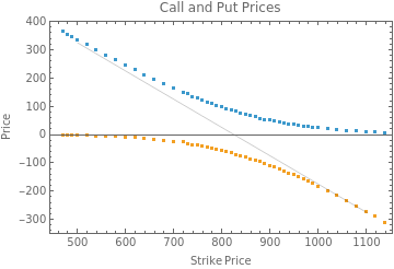
Here is the bid pricing for the October expiration option chain. It is obviously based on a formula and not trading. In the option markets like the bond markets prices are set by the dealers, but at least in the options market you can place limit orders and wait for the dealers to match your price.
In[]:=
octOpt=Select[Keys@calls,StringContainsQ[#,"2025-10-17"]&][[1]]
Out[]=
2025-10-17:165
In[]:=
callPrices={#[["strikePrice"]],#[["bid"]]}&/@Flatten[Values[calls[octOpt]],1];
In[]:=
puts=opts["putExpDateMap"];putPrices={#[["strikePrice"]],#[["bid"]]}&/@Flatten[Values[puts[octOpt]],1];
Put prices are shown as negative values to highlight the symmetry between puts and calls.
In[]:=
g0=Plot[curprice-k,{k,500,1100},PlotStyle->{Black,Thin}];g1=ListPlot[{callPrices,{#1,-#2}&@@@putPrices},PlotRange->All,Frame->True,FrameLabel->{"Strike Price","Price"},PlotLabel->"Call and Put Prices"];Show[g1,g0]
Out[]=
Fitting the option chain using Mathematica functions and Schwab API parameters.
Fitting the option chain using Mathematica functions and Schwab API parameters.
Here are the parameters available.
In[]:=
Keys@opts
Out[]=
{symbol,status,underlying,strategy,interval,isDelayed,isIndex,interestRate,underlyingPrice,volatility,daysToExpiration,dividendYield,numberOfContracts,assetMainType,assetSubType,isChainTruncated,callExpDateMap,putExpDateMap}
In[]:=
vol=opts["volatility"]/100intrate=opts["interestRate"]/100curprice=opts["underlyingPrice"]days=DateDifference[Today,StringSplit[octOpt,":"][[1]]][[1]]div=opts["dividendYield"]
Out[]=
0.29
Out[]=
0.0425
Out[]=
825.605
Out[]=
165
Out[]=
-1.
The minus 1. returned appears to be an error code. The dividend rate is from FinancialData[].
In[]:=
div=4QuantityMagnitude@FinancialData[ticker,"Dividend"]/curprice
Out[]=
0.0072674
In[]:=
americanCall[strike_?NumericQ,days_,intrate_,volatility_?NumericQ,dividend_,curprice_]:=FinancialDerivative[{"American","Call"},{"StrikePrice"strike,"Expiration"days/365},{"InterestRate"intrate,"Volatility"volatility,"CurrentPrice"curprice,"Dividend"dividend}];americanPut[strike_,days_,intrate_,volatility_,dividend_,curprice_]:=FinancialDerivative[{"American","Put"},{"StrikePrice"strike,"Expiration"days/365},{"InterestRate"intrate,"Volatility"volatility,"CurrentPrice"curprice,"Dividend"dividend}];
In[]:=
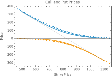
g2=Plot[{americanCall[k,days,intrate,vol,div,curprice],-americanPut[k,days,intrate,vol,div,curprice]},{k,500,1100}];
Here are the fits; they are not very good. The shape suggests that the volatility parameter is probably wrong.
In[]:=
Show[g1,g2,g0]
Out[]=
Black Scholes model to calculate volatility
Black Scholes model to calculate volatility
Black-Scholes fit with NonlinearModelFit[]
The fit is a may be a little off but on most runs performs well.
Curves using the Black-Scholes volatility calculation look much better.
Trying to trick NonlinearModelFit[] into using americanCall doesn’t work, even with starting point. Volatility comes out way too high.
CITE THIS NOTEBOOK
CITE THIS NOTEBOOK
Evaluating Schwab API option pricing: implied volatility and Black-Scholes analysis
by Robert Rimmer
Wolfram Community, STAFF PICKS, May 6, 2025
https://community.wolfram.com/groups/-/m/t/3455558
by Robert Rimmer
Wolfram Community, STAFF PICKS, May 6, 2025
https://community.wolfram.com/groups/-/m/t/3455558

