Two components are separated by liquid chromatography using the two-phase rate model and either the stagewise model (finite differences) or orthogonal collocation. Linear equilibrium is assumed. The derivation of the governing equation are available in Ref. 1 where this problem was originally solved using Berkeley-Madonna and the stagewise method. Here, we solve the same problem using Mathematica and the orthogonal collocation. Finally, we compare the results obtained using both numerical techniques.
Mass Transfer coefficients of components A and B
In[]:=
keffA=1.88 10^-4;
In[]:=
keffB=1.94 10^-4;
Péclet number
In[]:=
Pe=0.2/ϵ+0.011/ϵ (Ren/ϵ)^0.48
Out[]=
0.2
ϵ
0.011
0.48
Ren
ϵ
ϵ
Reynolds number
In[]:=
Ren=ρ L (4/(ϵ Pi Dc^2)) Dp/η
Out[]=
4DpLρ
2
Dc
Diffusivity
In[]:=
Di=L Dp 4/(Pe ϵ Dc^2 Pi)
Out[]=
4DpL
2
Dc
0.2
ϵ
0.0123523η
0.48
DpLρ
2
Dc
2
ϵ
ϵ
Nomenclature :
Packing particle diameter=Dp
Column diameter=Dc
Volumetric flow rate=L
Density of liquid phase=ρ
Viscosity of liquid phase=η
Void fraction of the bed=ϵ
Packing particle diameter=Dp
Column diameter=Dc
Volumetric flow rate=L
Density of liquid phase=ρ
Viscosity of liquid phase=η
Void fraction of the bed=ϵ
In[]:=
Dp=7.5 10^-3;
Dc=4;
L=0.4;
ρ=0.74;
η=2.2 10^-3;
ϵ=0.4;
Dc=4;
L=0.4;
ρ=0.74;
η=2.2 10^-3;
ϵ=0.4;
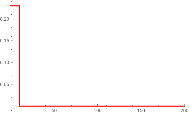
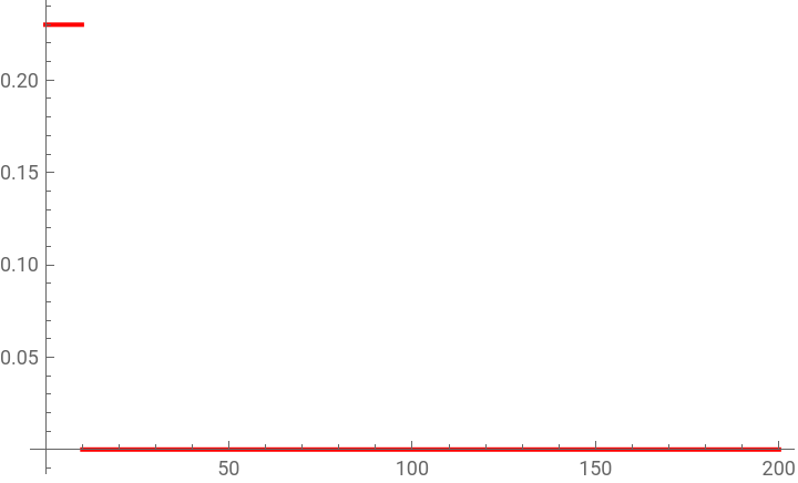
Injection of components A and B
In[]:=
CA
0
CA
init
In[]:=
CA
init
In[]:=
Plot[[t],{t,0,200},PlotStyleRGBColor[1,0,0]]
CA
0
Out[]=
In[]:=
CB
0
CB
init
In[]:=
CB
init
In[]:=
Plot[[t],{t,0,200},PlotStyleRGBColor[1,0,0]]
CB
0
Out[]=
Equilibrium constants of components A and B
In[]:=
K
A
In[]:=
K
B
Cross sectional area of the column
In[]:=
Ac=Pi Dc Dc/4
Out[]=
4π
Area to volume ratio of the solid phase spheres
In[]:=
ap=6/Dp
Out[]=
800.
Column length
In[]:=
Lbed=25;
length and number of a differential element
In[]:=
dz=Lbed/Ne
Out[]=
25
Ne
In[]:=
Ne=200;
Ingham’s method based on finite differences
Ingham’s method based on finite differences
Solid phase equilibrium concentrations of components A and B. We assume linear adsorption isotherms. Expressions of the transfer rates labelled QA and QB.
In[]:=
CSAeq
1
K
A
CA
1
In[]:=
CSBeq
1
K
B
CB
1
In[]:=
CSAeq
Ne
K
A
CA
Ne
In[]:=
CSBeq
Ne
K
B
CB
Ne
In[]:=
For[i=2,i<200,{[t]=keffA([t]-[t])(1-ϵ)ap/ϵ,[t]=[t],i=i+1}];
QA
i
CSAeq
i
CSA
i
CSAeq
i
K
A
CA
i
In[]:=
For[i=2,i<200,{[t]=keffB([t]-[t])(1-ϵ)ap/ϵ,[t]=[t],i=i+1}];
QB
i
CSBeq
i
CSB
i
CSBeq
i
K
B
CB
i
In[]:=
QA
1
CSAeq
1
CSA
1
In[]:=
QB
1
CSBeq
1
CSB
1
In[]:=
QA
Ne
CSAeq
Ne
CSA
Ne
In[]:=
QB
Ne
CSBeq
Ne
CSB
Ne
Components balances for solid and liquid phases
In[]:=
eqA[1]=D[[t],{t,1}]Di([t]-[t])/dz^2-L([t]+[t]-2[t])/(2dzϵAc)-[t];
CA
1
CA
2
CA
1
CA
2
CA
1
CA
0
QA
1
In[]:=
eqB[1]=D[[t],{t,1}]Di([t]-[t])/dz^2-L([t]+[t]-2[t])/(2dzϵAc)-[t];
CB
1
CB
2
CB
1
CB
2
CB
1
CB
0
QB
1
In[]:=
eqA[i_]:=D[[t],{t,1}]Di([t]-2[t]+[t])/dz^2-L([t]-[t])/(2dzϵAc)-[t]
CA
i
CA
i+1
CA
i
CA
i-1
CA
i+1
CA
i-1
QA
i
In[]:=
eqB[i_]:=D[[t],{t,1}]Di([t]-2[t]+[t])/dz^2-L([t]-[t])/(2dzϵAc)-[t]
CB
i
CB
i+1
CB
i
CB
i-1
CB
i+1
CB
i-1
QB
i
In[]:=
eqSA[1]=D[[t],{t,1}]keffAap([t]-[t]);
CSA
1
CSAeq
1
CSA
1
In[]:=
eqSB[1]=D[[t],{t,1}]keffBap([t]-[t]);
CSB
1
CSBeq
1
CSB
1
In[]:=
eqSA[i_]:=D[[t],{t,1}]keffAap([t]-[t])
CSA
i
CSAeq
i
CSA
i
In[]:=
eqSB[i_]:=D[[t],{t,1}]keffBap([t]-[t])
CSB
i
CSBeq
i
CSB
i
In[]:=
eqSA[Ne]=D[[t],{t,1}]keffAap([t]-[t]);
CSA
Ne
CSAeq
Ne
CSA
Ne
In[]:=
eqSB[Ne]=D[[t],{t,1}]keffBap([t]-[t]);
CSB
Ne
CSBeq
Ne
CSB
Ne
In[]:=
eqA[Ne]=D[[t],{t,1}]Di([t]-[t])/dz^2-L([t]-[t])/(dzϵAc)-[t];
CA
Ne
CA
Ne-1
CA
Ne
CA
Ne
CA
Ne-1
QA
Ne
In[]:=
eqB[Ne]=D[[t],{t,1}]Di([t]-[t])/dz^2-L([t]-[t])/(dzϵAc)-[t];
CB
Ne
CB
Ne-1
CB
Ne
CB
Ne
CB
Ne-1
QB
Ne
Solving the set of differential equations
In[]:=
Unknown=Join[Table[,{i,1,200}],Table[,{i,1,200}],Table[,{i,1,200}],Table[,{i,1,200}]];
CSA
i
CSB
i
CA
i
CB
i
In[]:=
initialCond=Join[Table[[0]0,{i,1,200}],Table[[0]0,{i,1,200}],Table[[0]0,{i,1,200}],Table[[0]0,{i,1,200}]];
CA
i
CB
i
CSA
i
CSB
i
In[]:=
eqn=Join[Table[eqA[i],{i,1,200}],Table[eqB[i],{i,1,200}],Table[eqSA[i],{i,1,200}],Table[eqSB[i],{i,1,200}]];
In[]:=
sys=Flatten[Join[eqn,initialCond]];
In[]:=
sol=NDSolve[sys,Unknown,{t,0,5000}];
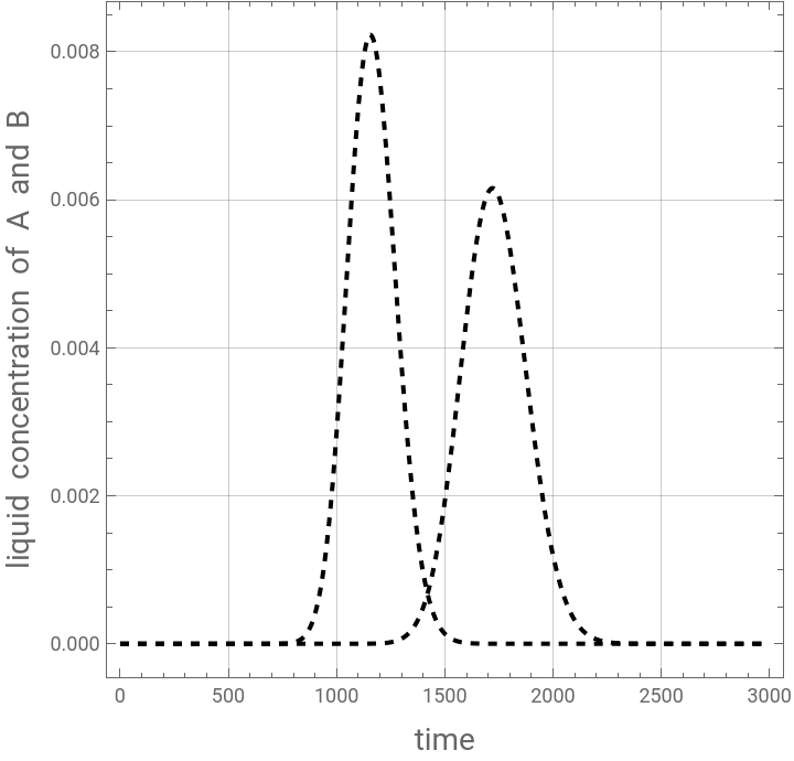
Plotting the profile of the concentration of components A and B at the exit of the column versus time. Peaks are quite symmetric because of the linear equilibrium assumption. Peak two is wider because its elution time is larger.
In[]:=
plt1b=Plot[Evaluate[[t]]/.sol,{t,0,3000},PlotRangeAll,PlotStyle{RGBColor[0,0,0],Dashed}];
CA
200
In[]:=
plt2b=Plot[Evaluate[[t]]/.sol,{t,0,3000},PlotRangeAll,PlotStyle{Dashed,RGBColor[0,0,0]}];
CB
200
In[]:=
Show[plt1b,plt2b,ImageSize-> Medium,AspectRatio-> 1,Frame-> True,GridLines->Automatic,
FrameLabel->{Style["time",14],Style["liquid concentration of A and B",14]}]
FrameLabel->{Style["time",14],Style["liquid concentration of A and B",14]}]
Out[]=
Our method based on orthogonal collocation and the Gauss-Lobatto nodes
In[]:=
ClearAll["CA*","CB*","QA[*","QB[*","CSA*","CSB*","eqA*","eqB*","eqS*"]
Chebyshev Derivative matrices (41 collocation points)
In[]:=
Np=40;d[0,0]=(2Np^2+1)/6//N;d[Np,Np]=-(2Np^2+1)/6//N;yc[i_]:=Cos[iPi/Np]//N;d[i_,i_]:=-yc[i]/(2(1-yc[i]^2))//N;d[j_,k_]:=If[j≠k&&k≠0&&k≠Np&&j≠0&&j≠Np,(-1)^(j+k)/(yc[j]-yc[k])]//N;d[Np,0]=-1/2(-1)^Np;d[0,Np]=1/2(-1)^Np;d[j_,0]:=If[j≠Np&&j≠0,-1/2(-1)^j/(1-yc[j])];d[j_,Np]:=If[j≠Np&&j≠0,1/2(-1)^(j+Np)/(1+yc[j])];d[0,j_]:=If[j≠Np&&j≠0,2(-1)^j/(1-yc[j])];d[Np,j_]:=If[j≠Np&&j≠0,-2(-1)^(j+Np)/(1+yc[j])];Add=Table[d[i,j]//N,{i,0,Np},{j,0,Np}];Bdd=Add.Add;
First-order and Second-order derivatives of CA and CB
Solid phase equilibrium concentrations of components A and B. We assume linear adsorption isotherms. Expressions of the transfer rates labelled QA and QB.
Components balances for solid and liquid phases
Solving the set of differential equations
In[]:=
eqn=Join[Table[eqA[i],{i,1,Np}],Table[eqB[i],{i,1,Np}],Table[eqSA[i],{i,1,Np+1}],Table[eqSB[i],{i,1,Np+1}]];
In[]:=
sys=Flatten[Join[eqn,initialCond]];
In[]:=
sol=NDSolve[sys,Unknown,{t,0,5000},AccuracyGoal -> 10];
Plotting the profile of the concentration of components A and B at the exit of the column versus time. Peaks are quite symmetric because of the linear equilibrium assumption. Peak two is wider because its elution time is larger.
In[]:=
Show[plt1,AspectRatio-> 1,Frame-> True,GridLines->Automatic,
FrameLabel->{Style["time",14],Style["liquid concentration of A and B",14]}]
FrameLabel->{Style["time",14],Style["liquid concentration of A and B",14]}]
Comparison between our method based on orthogonal colocation (colored lines) and Ingham' s method based on finite differences (black dashed lines)
In[]:=
Show[plt1,plt1b,plt2b,AspectRatio-> 1,Frame-> True,GridLines->Automatic,
FrameLabel->{Style["time",14],Style["liquid concentration of A and B",14]}]
FrameLabel->{Style["time",14],Style["liquid concentration of A and B",14]}]
References
References
◼
[1] J. Ingham, I. J. Dunn, E. Heinzle, J. E. Prenosil, J.B. Snape, Chemical Engineering Dynamics, Weinheim: Wiley - VCH, 2000
CITE THIS NOTEBOOK
CITE THIS NOTEBOOK
Liquid Chromatography with Linear Adsorption Equilibrium and Transfer Rate Model
by Housam Binous and Ahmed Bellagi
Wolfram Community, STAFF PICKS, March 19, 2024
https://community.wolfram.com/groups/-/m/t/3143304
by Housam Binous and Ahmed Bellagi
Wolfram Community, STAFF PICKS, March 19, 2024
https://community.wolfram.com/groups/-/m/t/3143304