In this computational essay we will explore multiway systems using complex numbers and plot them all in the complex plane. We will then analyze some patterns created by certain rules and prove them mathematically, find some novel fractals and prove them mathematically and end with some general results that we can classify our rules with and also prove them mathematically. We will be mainly focusing on conjugates as they are more likely to produce interesting results. These multiway systems, better known as holomorphic dynamical systems, can help us model chaotic systems like the weather or fluid motion.
Introduction
Introduction
An Introduction to Complex Numbers
An Introduction to Complex Numbers
It is essential that we familiarize ourselves with complex numbers and a multiway graph before we start our exploration of them. A complex number is an element of the number system that extends the real numbers with a specific element denoted with , called the imaginary unit, and satisfying the equation -1. Every complex number can be expressed in the form , where are real numbers.
i
2
z
a+bi
a,b
All basic arithmetic operations follow the same as those with real numbers. One very interesting property of complex numbers arise when multiplying two complex numbers.
By Euler we can represent any complex number as where is a real scaling variable and is the angle from the positive x-axis. By invoking properties of the unit circle we can easily also conclude that . Essentially this means that multiplying two complex numbers results in a rotation.
r
iθ
e
r
θ
rr(cos(θ)+isin(θ))
iθ
e
More formally if we have a complex number and complex number , both of which are on the unit circle, the multiplication by gives which is just a rotation of by .
a
i
θ
1
e
b
i
θ
2
e
b
ab
i(+)
θ
1
θ
2
e
a
θ
2
An Introduction to Multiway Systems
An Introduction to Multiway Systems
Multiway Systems and the Complex Plane
Multiway Systems and the Complex Plane
In this essay we will be examining a set of iterative function systems (IFS). To give a small example of an IFS we can consider the code snippet shown below.
Map :
n(in,4n)
In[]:=
ResourceFunction["NestGraphTagged"][n|->{(I)n,4n},1,6,"StateLabeling"->True, GraphLayout->{"LayeredDigraphEmbedding","RootVertex"->1}, PlotLegendsTraditionalForm/@{In,4n},PlotRange{{-7,7},{-1,9}}]
Out[]=
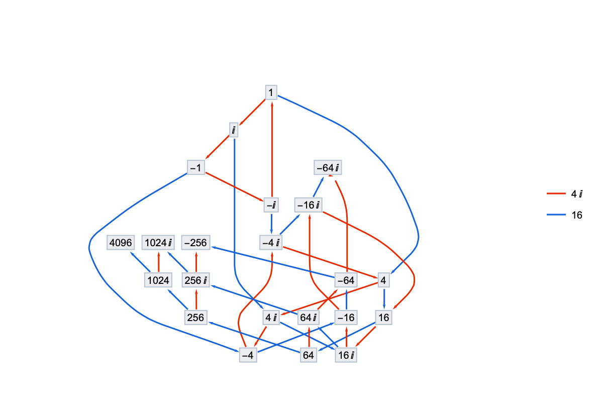
The above diagram shows mapping to and where starts from 1. We also used the Resource Function “NestGraphTagged” to draw our multiway systems. While this example was not drawn on the complex plane, it helps us to get an intuitive understanding of what a multiway system is. We do this because all our labels are complex numbers and it is natural to see what happens when we plot them on the complex plane. To see how the above system looks on the complex plane consider the graph below:
n
ni
4n
n
Map from above plotted on complex plane
In[]:=
GraphicsRow[With[{g1=ResourceFunction["NestGraphTagged"][n|->{(I)n,4n},1,6,"StateLabeling"->True]}, Graph[g1,VertexCoordinates(#->ReIm[#]&/@VertexList[g1])]], With[{g2=ResourceFunction["NestGraphTagged"][n|->{(I)n,4n},1,6,"StateLabeling"->False]}, Graph[g2,VertexCoordinates(#->ReIm[#]&/@VertexList[g2])]]]
Out[]=

The graph on the left shows the system plotted on the complex plane but it is cluttered with the labelling of the coordinates so we produce the exact same graph but the label of the coordinates turned off.
Mergers
Mergers
Another important concept of multiway systems are mergers. A merger is defined to be a node that can be reached by two distinct paths of edges. For example consider the multiway graph shown below. [1]
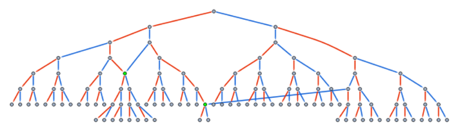
We can see two nodes which are highlighted green and these green points can be reached from the root vertex in two different ways. For example the left most green node can be reached by travelling along the following two paths RRRR and RBB and hence it is classified as a merger.
Why Study Complex Dynamics?
Why Study Complex Dynamics?
Complex dynamics was one of the original motivations for the study of fractal geometry, and it includes some of the most famous fractals in mathematics—the Julia sets and the Mandelbrot set. There are many applications of Complex Dynamics too. For example modeling any chaotic system like the motion of fluids to the solar system, the study of complex dynamics comes very handy.
The General Overview
The General Overview
In this computational essay we will start off by analyzing some patterns created by these multiway systems, then turn our attention to fractals, then focus on classifying sets of rules and finally future work for those interested.
Analyzing Patterns on Multiway Graphs
Analyzing Patterns on Multiway Graphs
Conjugated Stars
Conjugated Stars
One very interesting case to try is mapping which gives us star-like patterns which we will call conjugated stars. Note that we are working with conjugates mapping to two conjugates. For example let’s look at the example where we map to .
n((a+bi)n,(a-bi)n)
n
n
(10+8i)n,(10-8i)n
Conjugated Star mapping for 40 evolutions:
n((10+8i)n,(10-8i)n)
In[]:=
With[{g=ResourceFunction["NestGraphTagged"][n|->{(10+8I)n,(10-8I)n},1,40,"StateLabeling"->False]},GraphPlot[g,VertexCoordinates(#->ReIm[#]&/@VertexList[g])]]
Out[]=
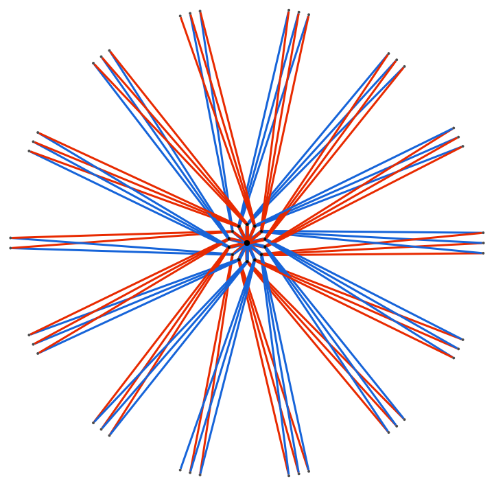
We can prove why this happens. Let’s define R to be the first rule (shown in red) and B to be the second rule (shown in blue). We claim that any order of R, B will take us to the same point.
In our case R is (10 + 8i)n and B is (10 - 8i)n.
For example RRB in the example shown is:
In our case R is (10 + 8i)n and B is (10 - 8i)n.
For example RRB in the example shown is:
1->(10+8i)->(10+8i)^2->(10+8i)^2(10-8i)
And RBR in the example is:
1->(10+8i)->(10+8i)(10-8i)->(10+8i)^2(10-8i)
The proof of this isn’t too hard to see from here. Since we are starting from 1 and multiplying either 10 + 8i or 10 - 8i, the order of multiplication does not matter and hence our claim is true.
This is not unique to the set and it works for any mapping of the form where is a complex number. For example we can run a similar mapping where . The reader is encouraged to change these parameters and explore.
This is not unique to the set
n((10+8i)n,(10-8i)n)
n(zn,n)
z
z
n((5+2i)n,(5-2i)n)
Conjugated Star mapping for 40 evolutions:
n((5+2i)n,(5-2i)n)
In[]:=
With[{g=ResourceFunction["NestGraphTagged"][n|->{(5+2I)n,(5-2I)n},1,40,"StateLabeling"->False]},GraphPlot[g,VertexCoordinates(#->ReIm[#]&/@VertexList[g])]]
Out[]=
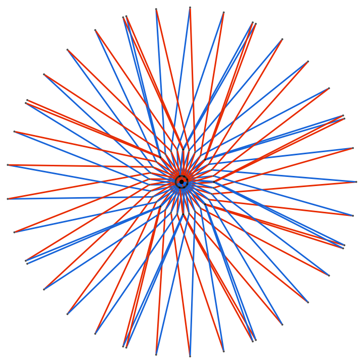
An interesting thing to note is that the conjugated stars above are not closed. For example if we look at the conjugated star above there are exactly two edges that only have degree of 1. This problem arises because we are running these IFS only a finite number of evolutions. If we were to run this for an infinite number of evolutions, it would make sense that the edges would eventually converge and the conjugated star would be closed.
One may also wonder how would these conjugated stars look on a plain multiway system that is not on the complex plane and what can we discover from that.
For example consider the code below:
Drawing out mergers on multiway system for conjugated star above:
In[]:=
g=ResourceFunction["NestGraphTagged"][n|->{(5+2I)n,(5-2I)n},1,6,"StateLabeling"->False,GraphLayout->{"LayeredDigraphEmbedding","RootVertex"->1}];mergers=Select[VertexList[g],VertexInDegree[g,#]>=2&];highlightedGraph=Graph[g,VertexStyle->Thread[mergers->Yellow]]
All the yellow points are mergers and this is useful for us because we can generate any conjugated star and we immediately know where the mergers must be. On the conjugated star, any vertex with a degree of 4 or more is considered a merger. Due to the number of evolutions, it is quite hard to see the colors on the conjugated star and hence why we will not produce those in this essay.
Spirals
Spirals
Drawing Spirals:
This result shouldn’t be too surprising because we are just rotating complex numbers as that is what multiplying two complex numbers means. When we don’t plot the graph on the complex plane we can expect a straight line as there is just one branch.
Drawing multiway system for Spiral above:
Clearly there are no mergers in this system as it is just a straight line.
Generating and Analyzing Fractals
Generating and Analyzing Fractals
Famous Fractals and a Variations
Famous Fractals and a Variations
There are many famous fractals but in this article we will explore the Sierpinski Triangle and the 3-Branch Tree Fractal. In some sense both of these fractals are versions of each other where the 3-Branch Tree Fractal is a broken Sierpinski Triangle that is pulled upward.
Sierpinski Triangle
Sierpinski Triangle
Let’s take a look at the Sierpinski Triangle. This was taken off from Stephen Wolfram’s “Multicomputation with Numbers: The Case of a Simple Multiway System.” [5] Below is the code:
Drawing Sierpinski Triangle using multiway system of order 3:
We will prove that this is actually a fractal but to do that we need to establish a few definitions.
Definition 2 (Hausdorff Dimension): The Hausdorff Dimension measures the roughness of a shape. For regular shapes like lines, squares, and cubes, their Hausdorff dimensions are the same as their familiar dimensions (1 for a line, 2 for a square, 3 for a cube). But for irregular shapes like clouds, coastlines, or fractals, the Hausdorff dimension might be a non-integer value, reflecting their intricate structure that lies somewhere between the traditional dimensions. [3]
Definition 3: A set is a fractal if its Hausdorff Dimension is strictly greater than the topological dimension.
Now that we are equipped with the terminology we can start to prove that the Sierpinski triangle is a fractal.
The boundary of these sets are the vertices of the smaller triangles. Thus the basis set has dimension 0 meaning that the Sierpinski Triangle has dimension 1. [2]
3-Branch Tree Fractal
3-Branch Tree Fractal
The 3-Branch Tree Fractal is a modification of the Sierpinski Triangle where we break it in the middle of the bottom edge and pull it upward in some sense. The below code shows how to produce the 3-Branch Tree Fractal and this was taken off from Stephen Wolfram’s “Multicomputation with Numbers: The Case of a Simple Multiway System.” [5]
Drawing 3-Branch Tree Fractal using multiway system of order 3:
Once again we can prove that this is truly a fractal by using the metrics defined above. The Hausdorff Dimension still remains the same as the Sierpinski’s Triangle because this fractal is essentially the same. The topological dimension also does not change and hence we can conclude that this must be a fractal.
Another Variation
Another Variation
This is another variation of the Sierpinski Triangle. While it has no official name, we will just call it Pulled Sierpinski.
Variations of Sierpinski Triangle on multiway system of order 3:
This example is more clear of what we mean by Pulled Sierpinski as we are literally pulling the Sierpinski Triangle. The proof that this is a fractal is the same as the one above so we won’t be explicitly writing it out.
The Leaf Fractal
The Leaf Fractal
Fractals are a core part of complex dynamics. There are many fractals that can be generated using an IFS. Two famous fractals are the Mandelbrot set and the Julia set. Though we won’t be exploring them directly in this computational essay we will draw heavy inspiration from them to generate our own fractals.
Drawing novel leaf fractal:
We will mathematically prove that this is a fractal. This means that we need to show that the Hausdorff Dimension is strictly greater than the topological dimension of our Leaf Fractal.
We can obtain a basis for the open set in the leaf by intersecting the leaf with images of T under the application of the function generated by IFS. Two such images are shown below and are outlined in blue.
Note that the boundary of these sets in the Leaf Fractal don’t intersect with the next evolution of the fractal and hence producing a null set which has topological dimension of -1 by definition. Hence our Leaf Fractal has topological dimension of 0 by definition 1.
Therefore our Leaf Fractal is fractal since the Hausdorff Dimension is greater than the topological dimension.
We can also analyze the mergers on this fractal. Consider the following code which highlights the mergers yellow:
Highlighting mergers on Leaf Fractal:
It is quite interesting that the mergers all are concentrated on the center leaf. If we look closely we can see that the center leaf is the merger because both of the diagonal leafs connect to it by the first two rules. While this is not a rigorous proof it serves the purpose for intuition. If we look more closely we can also see that there are no point which are triple mergers and we can verify this by using code:
Proving that Leaf Fractal doesn’t have mergers of InDegree 3:
Clearly there are no yellow points meaning that there are no triple or higher order mergers. We can prove this albeit not completely rigorously. Let’s try to prove this by contradiction.
Tree Fractals
Tree Fractals
There are many other fractals that we can generate with complex numbers. Let’s look at a classic fractal structure: the tree!
We will first look at a tree fractal that was produced by Stephen Wolfram. [5] Here the ComplexTreeGraphics function generates a tree fractal structure using IFS.
The diagram below shows how the tree fractal develops for 7 stages. This was taken off from Stephen Wolfram’s “Multicomputation with Numbers: The Case of a Simple Multiway System.” [5]
Drawing out 7 evolutions of tree fractal:
The proof that this is a fractal isn’t too hard as it follows the exact same logic as we followed for the leaf fractal. The proof is left as an exercise to the reader and it follows the exact same reasoning as the proofs above.
Another tree fractal can be obtained by slightly modifying the rules above:
Drawing out 10 evolutions of another tree fractal:
The proof of this is the exact same as the one above so if you figured the proof above you should also get this one!
Other Fractals
Other Fractals
We will devote this section to other fractals which look interesting. We won’t be proving them in this section but just adding them here so the viewer can enjoy them! One such fractal is produced using ComplexTreeGraphics.
Drawing Tree Fractal that looks like the border of the Koch Snowflake:
It is also very interesting that this fractal, though drawn with the ComplexTreeGraphics, doesn’t look like a tree. It seems to be bordering the Koch Snowflake. If we rotated this fractal all the way around we would end up with the Koch Snowflake. The mathematical reason behind this unknown and the curious reader is encouraged to explore this.
Another very cool fractal arises when we have a quadruple multiway system. We will call this fractal then Pentagon Swirl. The Pentagon Swirl is self contained which is also quite interesting and we will be analyzing these types of shapes in the next section.
Drawing Pentagon Swirl Fractal:
Adding Dynamic User Interface for Patterns
Adding Dynamic User Interface for Patterns
Using manipulate and bounding a, b, c so user can make their own patterns:
Drawing self contained fractals:
We can also enable State Labeling for a fewer number of evolutions so the reader can get a bigger overview of where the coordinates are.
The above Manipulate but with coordinates labelled:
Lastly, we come back to the generalized spiral. We conjecture that the code below always produces fractals. Once again, technically this is not considered as a multiway system but we will still classify it as such.
Conclusion
Conclusion
Throughout this article we explored patterns created by multiway systems of complex numbers. These patterns helped us understand how certain IFS behave on the complex plane. Then we created multiple fractals, a few famous ones and a few novel ones, and proved that they are fractals using rigorous mathematical proofs. Then we explored dynamical user interfaces to generalize patterns about a certain rule and made some observations about them. In this section we also left a few open problems for the interested reader. The purpose of this article was the discover what multiway systems with complex numbers could generate and as we know it we believe that these systems can generate many fractals making it an interesting tool for researchers to work with in the future.
Future Directions
Future Directions
Another possible avenue of exploration is to connect the multiway systems to the Julia set and Mandelbrot set. This was one of the initial goals of this research but I was not able to find any relations in the time of this research.
Sources
Sources
1
.Eric Archerman. (2023, July 13). On the mergers of numerical multiway systems. Wolfram Community. https://community.wolfram.com/groups/-/m/t/2965206
2
.M.Hatton & Mark McClure. (2022 February 13). What’s the topological dimension of Sierpiński’s triangle? Mathematics Stack Exchange. https://math.stackexchange.com/questions/4381051/whats-the-topological-dimension-of-sierpińskis-triangle
3
.Wikimedia Foundation. (2024, April 26). Hausdorff dimension. Wikipedia. https://en.wikipedia.org/wiki/Hausdorff_dimension
4
.Wikimedia Foundation. (2024, June 4). Lebesgue covering dimension. Wikipedia. https://en.wikipedia.org/wiki/Lebesgue_covering_dimension
5
.Wolfram, S., & Boyd, J. (2021, October 7). Multicomputation with numbers: The case of simple multiway systems-wolfram physics bulletins. Wolfram Physics Bulletins RSS. https://www.wolframphysics.org/bulletins/2021/10/multicomputation-with-numbers-the-case-of-simple-multiway-systems/#complex-numbers
Acknowledgements
Acknowledgements
I would like to thank my mentor Henry Gustafson for countless hours of help and guidance on my research, teaching me how to riffle shuffle cards, discovering new ways to tie shoelaces and posing interesting riddles and puzzles during breaks. I would also like to thank my group mates Austin Jiang and Joshua Yoo for their feedback on my project and for re-energizing me during the breaks and buying me ice-cream at Starbucks. I would like to thank all of my peers at Wolfram Summer Research Program for keeping me motivated and engaged in my research. I would also like to thank Stephen Wolfram for suggesting the project idea and the directors (Rory Foulger, Eryn Gillman, Megan Davis) for organizing the program. I would also like to thank all the TAs for running the social events so I could make many friends from this camp!
Lastly I would like to thank my parents and brother for their support and encouragement, especially through moments of homesickness during this program.
CITE THIS NOTEBOOK
CITE THIS NOTEBOOK
Exploring holomorphic dynamics with multiway systems
by Sambhu Ganesan
Wolfram Community, STAFF PICKS, July 12, 2024
https://community.wolfram.com/groups/-/m/t/3215155
by Sambhu Ganesan
Wolfram Community, STAFF PICKS, July 12, 2024
https://community.wolfram.com/groups/-/m/t/3215155