This project seeks to investigate sandpile models from the perspective of multiway systems, exploring how 1 and 2-dimensional configurations evolve under Bak-Tang-Wiesenfeld criteria in branchial space. While the final configurations of 1-dimensional initial lattices vary with respect to cyclical perturbations between minimally stable states, the outputs in 2 dimensions suggest a non-Abelian character. This is further explored via known formalisms that connect sandpile models to logarithmic conformal field theories capable of describing symplectic fermions with central charge ; the partition functions and correlation functions of scaling fields are discussed in this multiway lens.
c=-2
Introduction
Introduction
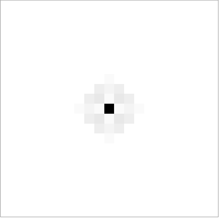
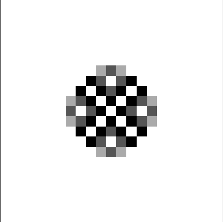
Sandpile models, a class of cellular automata, were first introduced by Per Bak, Choa Tang, and Kurt Wiesenfeld in 1987 [1]. With a single rule, we can see a version of it evolve deterministically as follows:
In[]:=
SandStep[s_]:=s+ListConvolve[{{0,1,0},{1,-4,1},{0,1,0}},UnitStep[s-4],2,0]ArrayPlot/@Take[NestList[SandStep,CenterArray[{{100}},{21,21}],100],1;;-1;;20]
Out[]=
,

,
,

,
,
Indeed, the configuration evolves toward a single ultimate state! With different initial conditions, we can see a different type of sandpile displacement occur with time progressing downwards:
In[]:=
SandStep1[s_]:=s+ListConvolve[{1,-2,1},UnitStep[s-2],2,0]ArrayPlot@Transpose[NestList[SandStep1,CenterArray[{10},21],40]]
Out[]=
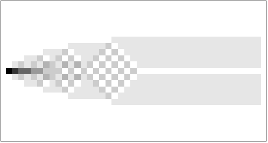
The same occurs here, as shown by the entire lower half of the plot! Applying the same evolution rule to a larger sandpile in a larger lattice, we can see the system cycle between a fixed set of recurrent configurations, which occur after the transient configurations of the earlier states:
In[]:=
ArrayPlot[Transpose[NestList[SandStep1,CenterArray[{41},21],200]],ColorFunction->"TemperatureMap"]
Out[]=

One defining property of the original Bak-Tang-Wiesenfeld sandpile model is its Abelian nature; due to how sandpiles topple upon exceeding a prescribed critical value , the number of stable configurations the system would vary between is substantially less than the number of total configurations. Using the multiway system capabilities of Wolfram Language, we can study this behavior more extensively by observing the entire ensemble of possible states in branchial space. This enables us to see different physical applications of the sandpile model—such as a 2-dimensional, logarithmic type of conformal field theory with central charge —in a new light.
z
c
c=-2
1-Dimensional Implementation
1-Dimensional Implementation
Here, we implement a multiway sandpile model in 1-dimension, using a list to represent a linear lattice:
In[]:=
ReplaceHeight1D[s_,vertex_,diff_]:=If[vertex<1||vertex>Length[s],s,ReplacePart[s,vertex s[[vertex]]+diff]];ChangeGrain1D[s_List,{}]:=s;ChangeGrain1D[s_List,vertexDiff_List]:=Module[{vertex,diff,newList}, vertex=Keys[vertexDiff[[1]]]; diff=Values[vertexDiff[[1]]]; newList=ReplaceHeight1D[s,vertex,diff]; ChangeGrain1D[newList, Rest[vertexDiff]] ];
We define some functions to check and enforce stability (each point on the lattice has associated height ):
h<=2⋅Dim[Sandpile]=2
z
c
In[]:=
IsStable[s_,zc_]:=AllTrue[s,#<zc&];Stabilize[s_,zc_]:=Module[{c,assoc,dec}, c = FirstPosition[s,_?(#≥zc&)][[1]]; assoc={c-2}~Join~Which[cLength[s],{(c-1)1},c1,{(c+1)1},True,{(c-1)1,(c+1)1}]; dec=ChangeGrain1D[s,assoc]; If[IsStable[dec,zc],dec,Stabilize[dec,zc]]];
A random possibility generator, as in a typical Abelian sandpile model that picks sites according to a specified probability distribution, is defined:
In[]:=
RandomPossibility[s_,zc_]:=Module[{rand,newList}, rand=RandomInteger[{1,Length[s]}]; newList=ChangeGrain1D[s,{rand1}]; If[IsStable[newList,zc],newList,Stabilize[newList,zc]] ];
Take[ArrayPlot[{#}]&/@NestList[RandomPossibility[#,2]&,{0,0,0,0},500],1;;-1;;80]
Out[]=
,

,

,
,
,

,

In the multiway model, we see that a minimally stable state is obtained such that every lattice site tends toward the critical slope:
In[]:=
PossibilityGenerator[s_,zc_]:=DeleteDuplicates[ Table[If[IsStable[ChangeGrain1D[s,{i1}],zc],ChangeGrain1D[s,{i1}],Stabilize[ChangeGrain1D[s,{i1}],zc]],{i,Length[s]}]];Gen1DSandpile[s_,zc_]:=If[Depth[s]2,PossibilityGenerator[s,zc],Gen1DSandpile[#,zc]&/@s];
In[]:=
ResourceFunction["NestGraphTagged"][Gen1DSandpile[#,2]&,{{0,0,0,0,0,0}},11]
Out[]=
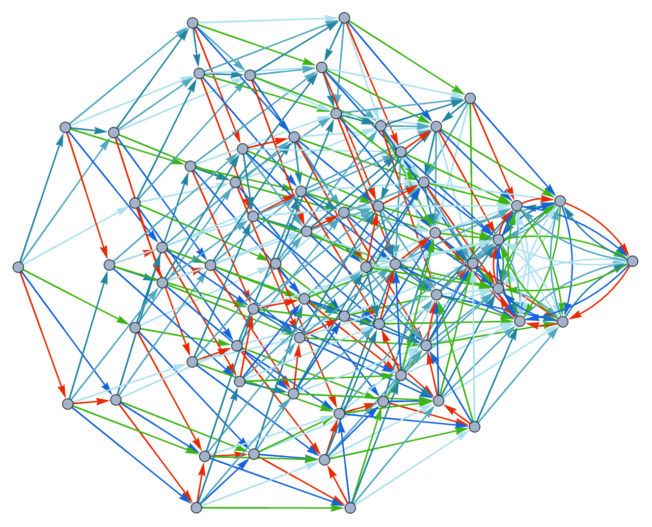
We can observe the branching behavior of the 1-dimensional multiway system in a graph distance matrix:
2-Dimensional Implementation
2-Dimensional Implementation
We now use matrices to represent square lattices for the 2-dimensional multiway sandpile model implementation:
We can manipulate sandpile heights like so:
For instance, we can stabilize an initially unstable 11x11 configuration with two critical sandpiles at its center:
We can generate random possibilities like so, as in a typical 2-dimensional Abelian sandpile model:
To generate all possibilities of a given configuration, we take:
Indeed, 2-dimensional lattices appear to evolve in branchial space under sandpile model criteria in a non-Abelian manner.
Applications to Logarithmic Conformal Field Theory
Applications to Logarithmic Conformal Field Theory
MaTeX Setup
MaTeX Setup
LCFT Discussion
LCFT Discussion
Sandpile model have been applied to numerous situations across numerous research topics; these include non-equilibrium statistical physics, quantum gravity, and plasma physics. Of interest is a proposed connection to a Gaberdiel-Kausch conformal field theory, which is rational with respect to its extended symmetry (triplet) algebra and permits correlators to be logarithmic at short distance scales as opposed to exponential [2]. (In other words, the dilation operator is non-diagonalizable.) To assemble such a local field theory description as outlined in [3], we define a discrete Laplacian for the sandpile model based on toppling behavior:
This matrix can be generated for an NxN square lattice:
We can first examine the asymptotic behavior of the free energy, which will also clarify why correlators behave logarithmically in the sandpile model. A more tangible partition function exists if we make the boundary conditions mixed; that is, we leave two edges open to toppling sites and the other two closed. For a square of size NxN, this is:
We can demonstrate a system like this by adjusting the system criteria:
As a layered digraph, this looks like the following:
Conclusion and Future Direction
Conclusion and Future Direction
Acknowledgements
Acknowledgements
I would like to thank Kurt Gimbel for his mentoring, as well as James Boyd for his idea of evolving and analyzing a multiway sandpile model.
Citations
Citations
[1] P. Bak, C. Tang, and K. Wiesenfeld, Phys. Rev. Lett. 59, 381 (1987).
[2] Matthias R. Gaberdiel, Horst G. Kausch: “A Local Logarithmic Conformal Field Theory”, 1998, Nucl.Phys.B538:631-658,1999; arXiv:hep-th/9807091. DOI: 10.1016/S0550-3213(98)00701-9.
[3] S. Mahieu, P. Ruelle: “Scaling fields in the two-dimensional abelian sandpile model”, 2001, Phys.Rev. E64 (2001) 066130; arXiv:hep-th/0107150. DOI: 10.1103/PhysRevE.64.066130.
[4] S.N. Majumdar and D. Dhar, J. Phys. A: Math. Gen. 24, L357 (1991).