CITE THIS NOTEBOOK: Benchmarking numerical differential equations in Wolfram Language by Hanfeng Zhai. Wolfram Community DEC 12 2022.
CITE THIS NOTEBOOK: Benchmarking numerical differential equations in Wolfram Language by Hanfeng Zhai. Wolfram Community DEC 12 2022.
The Linear Convection Equation
The Linear Convection Equation
The simplest and most accessible equation in computational fluid dynamics (CFD) or more general partial differential equations (PDEs) should be the linear convection equation (LCE), i.e., the wave equation. Solving this equation with finite differences schemes is usually the first step for CFD (or more general applied math) beginners. Here, we demonstrate and compare the simple numerical solution schemes of such equations in Wolfram Language by comparing the Wolfram built-in functions, i.e., DSolve and NDSolve, and finite differences, i.e., with forward differences, backward differences, & central differences. This blog/tutorial mainly serves for educational purposes, for differential equations (DEs) beginners to better understand solutions of ODEs and further PDEs with numerical implementations. Note that the forward differences finite differences implementation are adapted and inspired from the famous Python code 12 Steps to CFD by Prof. Lorena Barba.The linear convection equation(s) write:+c0where c is the parameter to be given, u is the solution, x and t are the spatial and temporal domains, respectively. At , one have the initial condition(s) (ICs): Given this ICs, if we replace the variable as , and we further define ; then the LCE reduces to a simple ODE: 0. We hence have the exact (analytical) solution:
∂u
∂t
∂u
∂x
t0
u(x,0)(x)
u
0
x-ct
y
v(y,t):u(y+ct,t)
dv
dy
u(x,t)(x-ct)
u
0
Now, we solve this DE using the aforementioned methods for benchmarking and a better understanding of numerical PDEs.
Solve LCE using Wolfram Built-in Solver
Solve LCE using Wolfram Built-in Solver
Wolfram Language provides rich libraries to solve differential equations. Analytically and numerically, we can use DSolve and NDSolve to get the solutions. Now we demonstrate the two approaches to obtain the corresponding solutions.
Now, we try to solve the equation symbolically using NDSolve.
First, we can use DSolve to obtain the analytical (or symbolic) solution. Given the constant. We first define the PDE in the symbolic form:
Now, we try to solve the equation symbolically using NDSolve.
First, we can use DSolve to obtain the analytical (or symbolic) solution. Given the constant
c1
In[]:=
c=1;pdewave=D[u[x,t],t]+cD[u[x,t],x]==0
Out[]=
(0,1)
u
(1,0)
u
To get the solution, we simply recall the DSolve module:
In[]:=
solnwave=DSolve[pdewave,u[x,t],{x,t}]
Out[]=
{{u[x,t][t-x]}}
1
We are lucky to some since the 1D linear convection has an analytical solution. However, most of the existing PDEs does not have such a solution. Hence, numerically solve this is essential. We here first demonstrate the method with the built-in function NDSolve. We first define the initial condition (ICs) as a function :
f(x)
In[]:=
f[x_]:=-Sin[5x-Pi/2]
We can also visualize this initial condition:
In[]:=
Plot[-Sin[5x-Pi/2],{x,0,2},FillingAutomatic]
Out[]=
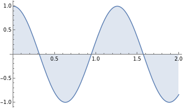
How to interpret this so-called ICs? We can think of the PDE as a "process". Given an initial state, the process will bring "it" (initial state) to "somewhere else", i.e. a final state. The ICS is this initial state, and the PDE, i.e. the wave equation, to take it to a final state to be solved. Numerical discretization can approximate this process.
To get solution, we recall the NDSolve module with also setting the boundary conditions (BCs):
In[]:=
mysol=NDSolve[{D[u[x,t],x]+D[u[x,t],t]==0,u[x,0]==f[x],u[0,t]==1},u[x,t],{x,0,2},{t,0,1}]
Out[]=
u[x,t]InterpolatingFunction[x,t]


We can then visualize the results in the 3D surface plot:
In[]:=
Plot3D[Evaluate[u[x,t]/.%],{x,0,2},{t,0,1},PlotRangeAll,ColorFunction"BlueGreenYellow"]
Out[]=

In[]:=
DensityPlot[Evaluate[u[x,t]/.%],{t,0,1},{x,0,2},ColorFunction"BlueGreenYellow",PlotLegendsAutomatic,AspectRatio1/2]
Out[]=
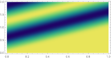

Pretty cool, huh! This 3D surface plot visualizes our prementioned "process" - how the solution operator takes the initial state to a final state with regard to both space ( here ) and time ( here ). You may also notice the surface contour looks pretty much like a wave, and that's why it's called the wave equation. Now we can switch some other cool ICs and see how the LCE solutions behave.
x
t
We can also switch some ICs and see how the solution behaves. For example, taking the initial function as
f(x)+1.9-
x
e
10
2
(x-1)
In[]:=
Plot[-(x-1)^2+1.9+Exp[x]/10,{x,0,2},PlotStyleBlue,FillingAutomatic]
Out[]=
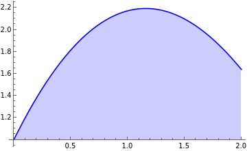
Enforce this function as the ICs and solve the wave equation, we can visualize the results as follows:
In[]:=
fic[x_]:=-(x-1)^2+1.9+Exp[x]/10
In[]:=
msol1=NDSolve[{D[u[x,t],x]+D[u[x,t],t]==0,u[x,0]==fic[x],u[0,t]==1},u[x,t],{x,0,2},{t,0,1}];
In[]:=
DensityPlot[Evaluate[u[x,t]/.%],{t,0,1},{x,0,2},ColorFunction"BlueGreenYellow",PlotLegendsAutomatic,AspectRatio1/2]
Out[]=
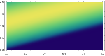

Which shows how the PDE "drives" this single wave to decay outside our solution region.
However, if we increase the order of the function, e.g. switch 2 to 16, we first visualize our ICs:
In[]:=
Plot[-(x-1)^16+1.9+Exp[x]/10,{x,0,2},PlotStyleBlue,FillingAutomatic]
Out[]=
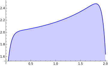
Solving the PDE we can see something interesting happening:
Then we observe a little "wavy behavior" of the discretized solution, which should not be expected. Why is this happening? It could be the discretization errors in NDSolve due to its employed discretization methods, i.e. discretization error. There could also be my hardware system problems, i.e., round-off errors. If you are excited about the specific reasons, feel free to read more here. Also, let me know if there are interests in related error analysis and I can further write a blog about this!
So, now, I will implement different finite difference schemes to solve the LCE and benchmark the solution processes!
Solve LCE using Explicit Numerical Discretization
Solve LCE using Explicit Numerical Discretization
In finite difference methods (FDM), the computational domain is discretized on a rectangular grid to obtain the numerical value on each node, i.e. intersections of the grids. Generally, FDM can be categorized into forward differences (FD), backward differences (BD) and central differences (CD).
Backward Differences Scheme
Backward Differences Scheme
Defining the computational domain:
Before defining the basis (nominated as xx), we first assign it with a constant array
Defining the ICs, which will be further propagating to a "solution", as usol:
Now, we define a solution matrix, the solution operator, i.e. how the ICs propagate in the spatiotemporal domain is stored in this matrix:
And we can solve the PDE given our discretization form written in a double for-loops, in which the discretized solution operator is stored in the SolMat:
Obtaining the discretized solutions, we can then visualize how to "wave" propagates w.r.t time in the spatial domain. If take 0.1 as the time interval, the visualization shows as follows:
Of course we can decrease the discretization intervals for better solution approximations:
Obtain the solution and plot its changes of spatial distribution w.r.t. time.
Plot the solution operator projected in the spatiotemporal domain:
In this case,the approximated solutions are much smoother. Comparing this with our previous solutions with NDSolve we can conclude that NDSolve discretization should be more complex than our vanilla BD schemes, with a smooth gradient transition observed.
We can then visualize how the spatial distribution of the solution evolve w.r.t. time:
And now we don't have the "wavy behavior" in the solution operator of our PDE! The initial wave gradually propagates outside the computational domain.
Another cool thing with the "hands-on" numerical discretization is that we can encode complex ICs for solutions. A good (and classic) example would be the complex square waves:
We first clear the memory space, define the variables, and define our complex initial square waves condition:
Solving this scenario with our vanilla BD we can then plot both the solution propagation w.r.t. time and its projection in the spatiotemporal domain:
Since this is a special case that specifically employed for our "hands-on" discretization, we use a different cool visualization method:
Looks pretty cool huh! The hands-on implemented finite difference schemes can give us an approximated solution for the sharp wavy ICs.
Forward Differences Scheme
Forward Differences Scheme
Let's apply this scheme to our previous employed case used for NDSolve. The implementation is simple:
Double-check it looks the same as our previous ICs; and then approximate use the forward difference scheme:
Discretize and solve the numerical solution:
And now the FD successfully obtain the numerical solutions!
Giving the IC as a higher order differential equation, we can also approximate the solution.
Central Differences Scheme
Central Differences Scheme
Benchmarking Solution Schemes
Benchmarking Solution Schemes
Since both BD, FD, and CD are (or are expected to) be able to approximate the solution with the sharp square wave ICs. We can now benchmark the spatiotemporal solutions obtained from both three methods and check the difference.
A higher order or sharp ICs may lead to the unstable solution of NDSolve.
One should be very careful about the finite difference schemes considering different equation parameters.
In the case of LCE, backward and forward differences require positive and negative, respectively, to make the approximated solutions stable.
Central differences are generally not stable for LCE. However, one can still obtain a converged numerical solution when the parameter is close to zero.
NDSolve is generally more stable w.r.t. to different kinds of PDEs as we do not need much prior knowledge regarding the equations to be solved.
References
References