Hello readers! Today I'm going to share this screen saver animation made from slice density plot and color arithmetic.
As usual some helper functions:
ClearAll[pipe,branch,branchSeq]pipe=RightComposition;branch=Through@*{##}&;branchSeq=pipe[branch[##],Apply[Sequence]]&;
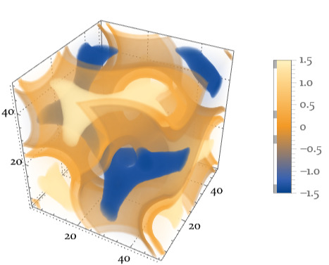
Starting out with the good old implicit surface (see Neat Examples in ContourPlot3D’s documentation):
In[]:=
densF=Compile[{x,y,z},Cos[x]Sin[y]+Cos[y]Sin[z]+Cos[z]Sin[x],RuntimeAttributes{Listable},RuntimeOptions"Speed",ParallelizationTrue,CompilationTarget"C"]
Out[]=

Subdivide[-π,π,50]//pipe[N,Outer[List,#,#,#]&,Transpose[#,{2,3,4,1}]&,Apply@densF,ListDensityPlot3D[#,PlotTheme"Detailed"]&]
I generate a 3D loop track (a closed B-spline) that looks kind of like a roller coaster:
(See code for cyclicBSpline and cyclicBSplineD at the end of the post.)
track=Module[{cptN=8,degree=4,cpts,bsf,bsfT,bsfdT},cpts=CirclePoints[{1,0},cptN](RandomReal[{.5,1},cptN]//Rescale[#,MinMax@#,π{.8,1}]&)//Transpose//Map[Rescale[#,MinMax@#,π{-1,1}]&]//Append[RandomReal[{-1,1},cptN]//Rescale[#,MinMax@#,{-1,1}]&]//Transpose//Echo[#,"cpts",Iconize[#,"cpts"]&]&;bsf=cyclicBSpline[cpts,degree];bsfT=cyclicBSplineD[cpts,degree,1];bsfdT=cyclicBSplineD[cpts,degree,2];Compile[{u},#[u],CompilationOptions{"InlineCompiledFunctions"->True,"InlineExternalDefinitions"True},RuntimeAttributes{Listable},ParallelizationTrue,RuntimeOptions"Speed",CompilationTarget"C"]&/@{bsf,bsfT,bsfdT}]
»
cpts
Out[]=
In[]:=
N@Subdivide[0,1,100]//Most//pipebranch@@track,MapThread[Function[{p,T,dT},{Cross[dT,T]//branchSeq[Cross[#,T]&,Identity],T}//Map@pipe[Normalize,{p,p+0.5#}&]],#,1]&,Transpose,Graphics3DAbsoluteThickness[.6],Red,Line@#1,Darker@Green,Line@#2,Blue,Line@#3,Black,//Append[#,#〚1〛]&//Line,&
Out[]=

Next, I place 500 rectangular slices along the loop. The loop goes through the center of each slice, and each slice is perpendicular to the loop:
In[]:=
Needs["Developer`"]
In[]:=
coords=N@Subdivide[0,1,500]//Most//pipe[branch@@track,MapThread[Function[{p,T,dT},Cross[dT,T]//branch[Cross[#,T]&,Identity]//Map@Normalize//Prepend[p]],#,1]&,Transpose[#,{3,1,2}]&(*<-{p,n,bn}*),ToPackedArray];grid=Outer[List,(*x:*)N@Most@Subdivide[-1,1,320],(*y:*)N@Most@Subdivide[-1,1,180]]//ToPackedArray;grid3d=Withscale=,grid.coords{2,3}//coords1+scaleTranspose[#,{3,4,1,2}]&//Transpose[#,{4,1,2,3}]&;
π
2
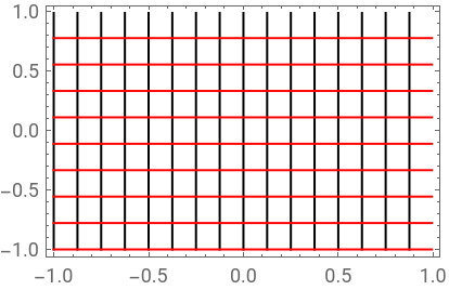
Base grid:
In[]:=
Graphics{Line[grid〚1;;-1;;20,{1,-1}〛],Red,Line[grid〚1;;-1;;20,{1,-1}〛]},FrameTrue,AspectRatio
320
500
Out[]=
3D grids on rectangular slices:
Block{coords,grid,grid3d},coords=N@Subdivide[0,1,50]//Most//pipe[branch@@track,MapThread[Function[{p,T,dT},Cross[dT,T]//branch[Cross[#,T]&,Identity]//Map@Normalize//Prepend[p]],#,1]&,Transpose[#,{3,1,2}]&,ToPackedArray];grid=Outer[List,(*x:*)N@Most@Subdivide[-1,1,11],(*y:*)N@Most@Subdivide[-1,1,11]]//ToPackedArray;grid3d=Withscale=,grid.coords{2,3}//coords1+scaleTranspose[#,{3,4,1,2}]&//Transpose[#,{4,1,2,3}]&;;Graphics3D{AbsoluteThickness[.6],Opacity[.6],LCHColor[0.7,0.7,0.2],Join[grid3d〚1;;-1;;2,;;,{1,-1}〛,grid3d//Transpose[#,{1,3,2,4}]&//#〚1;;-1;;2,;;,{1,-1}〛&]//Flatten[#,1]&//Line},//Show[#,N@Subdivide[0,1,100]//track〚1〛//Graphics3D[{Thick,LCHColor[0.55,1.04,0.35],Line@#}]&]&
π
4
I then calculate the density plot on each slice through densF, a bit like what the built-in SliceDensityPlot3D does:
That gives me 500 density image of the same dimensions:
Here comes the interesting part. Take some neighboring slices (e.g. slice 1-30) and use the visible spectrum to colorize them. Sum up the result in XYZ color space to derive a single image:
Do the same for next batch of neighboring slices (slice 2-21) to get the next image and so on:
All done! Now playing the frames to see my screen saver in its full glory:
Cyclic B-spline
Cyclic B-spline
i.e. a compiled version of BSplineFunction[cpts, SplineDegreedegree, SplineClosedTrue] :
Derivative of cyclic B-spline against parameter (which is another cyclic B-spline):