Introduction
Introduction
In this notebook we show the conversion of the Jupyter notebook used in the presentation "Monte Carlo Integration" by Vadim Smolyakov, [VSv1], into a Mathematica notebook. The Jupyter notebook, [VSn1], uses Python, the corresponding Mathematica notebook uses Wolfram Language (WL). We show how the conversion can be done using Large Language Models (LLMs) and how dedicated software packages can be used. (For the latter see [AAv1, AAv2].) For a more extensive discussion on notebook conversions see the blog post “Notebook conversions”, [AA1].
Links to videos
Links to videos
Original Monte-Carlo presentation
Original Monte-Carlo presentation
Conversion presentation
Conversion presentation
Programmatic conversion
Programmatic conversion
Ingestion
Ingestion
In[]:=
nbJupyter=Import["~/MathFiles/Community/monte_carlo_pi.ipynb","Text"]
LLM invocation
LLM invocation
In[]:=
res=LLMSynthesize[{"Convert the following Jupyter notebook into a Mathematica notebook:",nbJupyter,LLMPrompt["NothingElse"]["WL"]},LLMEvaluator->LLMConfiguration["Model"->"gpt-4-0125-preview"]]
Out[]=
```mathematica\n(* Monte Carlo Integration *)\n\n(* Suppose we want to evaluate an integral I = \int_{a}^{b} f(x) dx we can approximate the integral as follows *)\n\n(* I = \int_{a}^{b} f(x) dx = \int_{a}^{b} w(x) p(x) dx = E_p [w(x)] = \frac{1}{n} \sum_{i=1}^{N} w(x_i), where x_i \sim \mathrm{Unif}(a,b) *)\n\n(* We defined w(x) = f(x)(b-a) and p(x) = 1/(b-a) is the pdf of a uniform random variable over (a,b). As we increase the number of samples N, our empirical estimate of the mean becomes more accurate. In fact, the standard error is equal to \sigma/\sqrt{n}, where \sigma is the empirical standard deviation: *)\n\n(* \sigma^{2} = \frac{1}{N-1} \sum_{i=1}^{N} (f(x_i) - I)^{2} *)\n\n(* We can use a monte carlo integration to estimate \pi. We know that the area of a circle with radius r is \pi r^2. Alternatively, the area of a circle can be computed as: *)\n\n(* I = \int_{-r}^{r} \int_{-r}^{r} 1[x^2 + y^2 \leq r^2] dx dy = E_{x,y}[w(x,y)] *)\n\n(* Therefore, \pi = I / r^2. To compute I, note that: *)\n\n(* w(x,y) = (b_x-a_x)(b_y-a_y)1[x^2+y^2\leq r^2] = (2r)(2r)1[x^2+y^2\leq r^2] = 4r^2 1[x^2+y^2\leq r^2] *)\n\n(* where 1[x^2+y^2\leq r^2] is an indicator function equal to 1 when a point is inside a circle of radius r and equal to 0 otherwise. We can implement \pi estimator as follows. *)\n\nSeedRandom[42]; (* Ensuring replicability *)\n\nradius = 1;\nnumIter = 10^4;\n\nX = RandomReal[{-radius, radius}, numIter];\nY = RandomReal[{-radius, radius}, numIter];\n\nR2 = X^2 + Y^2;\ninside = UnitStep[radius^2 - R2];\noutside = 1 - inside;\n\nsamples = 4*radius^2*inside; (* Defining weighing function w(x, y) *)\n\nIHat = Mean[samples];\npiHat = IHat/radius^2;\npiHatSE = StandardDeviation[samples]/Sqrt[numIter];\n\nPrint["pi est: ", piHat, " +/- ", piHatSE];\n\n(* Visualizing Results *)\n\nGraphics[{\n {Red, Point[Transpose[{X, Y}] [[Flatten[Position[outside, 1]]]]]},\n {Blue, Point[Transpose[{X, Y}] [[Flatten[Position[inside, 1]]]]]}\n }, Frame -> True]\n```
In[]:=
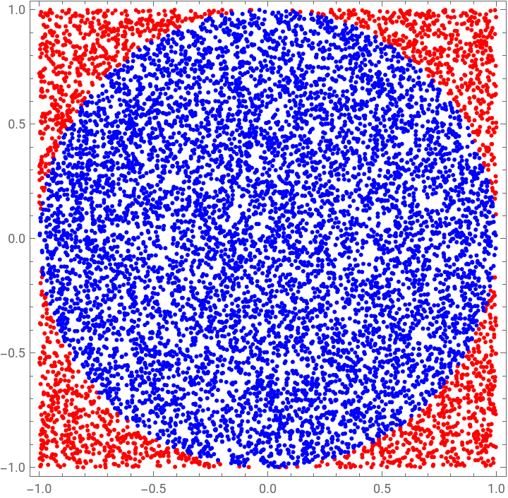
SeedRandom[42];(*Ensuringreplicability*)radius=1;numIter=10^4;X=RandomReal[{-radius,radius},numIter];Y=RandomReal[{-radius,radius},numIter];R2=X^2+Y^2;inside=UnitStep[radius^2-R2];outside=1-inside;samples=4*radius^2*inside;(*Definingweighingfunctionw(x,y)*)IHat=Mean[samples];piHat=IHat/radius^2;piHatSE=StandardDeviation[samples]/Sqrt[numIter];Print["pi est: ",piHat," +/- ",piHatSE];Print["pi est: ",N@piHat," +/- ",N@piHatSE];(*VisualizingResults*)Graphics[{{Red,Point[Transpose[{X,Y}][[Flatten[Position[outside,1]]]]]},{Blue,Point[Transpose[{X,Y}][[Flatten[Position[inside,1]]]]]}},Frame->True]
pi est: +/-
1573
500
61061
101
1500
pi est: 3.146 +/- 0.0163919
Out[]=
Using NIntegrate
Using NIntegrate
Monte-Carlo integration using NIntegrate:
In[]:=
NIntegrate[UnitStep[radius^2-(+)],{x,-radius,radius},{y,-radius,radius},Method->"MonteCarlo",PrecisionGoal->2]
2
x
2
y
Out[]=
3.10621
Collect the sampling points the during the Monte-Carlo integration that uses approximately the same number of sampling points as the LLM derived code above:
In[]:=
res=Reap@NIntegrate[UnitStep[radius^2-(+)],{x,-radius,radius},{y,-radius,radius},Method->"MonteCarlo",PrecisionGoal->5,EvaluationMonitor:>Sow[{x,y}],MaxPoints->numIter];
2
x
2
y
In[]:=
{numIter,res〚2,1〛//Length}
Plot of the sampling points:
In[]:=
ListPlot[GatherBy[res〚2,1〛,UnitStep[radius^2-#.#]&],AspectRatio->Automatic,PlotStyle->PointSize[0.01]]
Out[]=
Ad hoc theoretical text conversion
Ad hoc theoretical text conversion
Convert the following Markdown and code into WL code. Make sure the formulas are given as WL formulas.
Suppose we want to evaluate an integral I = \int_{a}^{b} f(x) dx we can approximate the integral as follows
I = \int_{a}^{b} f(x) dx = \int_{a}^{b} w(x) p(x) dx = E_p [w(x)] = \frac{1}{n} \sum_{i=1}^{N} w(x_i) , where x_i \sim \mathrm{Unif}(a,b)
We defined w(x) = f(x)(b-a) and p(x) = 1/(b-a) is the pdf of a uniform random variable over (a,b) . As we increase the number of samples N , our empirical estimate of the mean becomes more accurate. In fact, the standard error is equal to \sigma/\sqrt{n} , where \sigma is the empirical standard deviation:
\sigma^{2} = \frac{1}{N-1} \sum_{i=1}^{N} (f(x_i) - I)^{2}
We can use a monte carlo integration to estimate \pi . We know that the area of a circle with radius r is \pi r^2 . Alternatively, the area of a circle can be computed as:
I = \int_{-r}^{r} \int_{-r}^{r} 1[x^2 + y^2 \leq r^2] dx dy = E_{x,y}[w(x,y)]
Therefore, \pi = I / r^2 . To compute I , note that:
w(x,y) = (b_x-a_x)(b_y-a_y)1[x^2+y^2\leq r^2] = (2r)(2r)1[x^2+y^2\leq r^2] = 4r^2 1[x^2+y^2\leq r^2]
where 1[x^2+y^2\leq r^2] is an indicator function equal to 1 when a point is inside a circle of radius r and equal to 0 otherwise. We can implement \pi estimator as follows.
L
A
TE
XL
A
TE
X
Suppose we want to evaluate an integral I = \int_{a}^{b} f(x) dx we can approximate the integral as follows
I = \int_{a}^{b} f(x) dx = \int_{a}^{b} w(x) p(x) dx = E_p [w(x)] = \frac{1}{n} \sum_{i=1}^{N} w(x_i) , where x_i \sim \mathrm{Unif}(a,b)
We defined w(x) = f(x)(b-a) and p(x) = 1/(b-a) is the pdf of a uniform random variable over (a,b) . As we increase the number of samples N , our empirical estimate of the mean becomes more accurate. In fact, the standard error is equal to \sigma/\sqrt{n} , where \sigma is the empirical standard deviation:
\sigma^{2} = \frac{1}{N-1} \sum_{i=1}^{N} (f(x_i) - I)^{2}
We can use a monte carlo integration to estimate \pi . We know that the area of a circle with radius r is \pi r^2 . Alternatively, the area of a circle can be computed as:
I = \int_{-r}^{r} \int_{-r}^{r} 1[x^2 + y^2 \leq r^2] dx dy = E_{x,y}[w(x,y)]
Therefore, \pi = I / r^2 . To compute I , note that:
w(x,y) = (b_x-a_x)(b_y-a_y)1[x^2+y^2\leq r^2] = (2r)(2r)1[x^2+y^2\leq r^2] = 4r^2 1[x^2+y^2\leq r^2]
where 1[x^2+y^2\leq r^2] is an indicator function equal to 1 when a point is inside a circle of radius r and equal to 0 otherwise. We can implement \pi estimator as follows.

Programmatic conversion to Markdown
Programmatic conversion to Markdown
We can use LLMs to convert the Jupyter notebook into Markdown:
Here we export the result into a file:
References
References
◼
◼
◼
[AAv1] Anton Antonov, "Markdown to Mathematica converter (CLI and StackExchange examples)" , (2022), Anton A. Antonov's channel at YouTube .
◼
[AAv2] Anton Antonov, "Markdown to Mathematica converter (Jupyter notebook example)" , (2022), Anton A. Antonov's channel at YouTube .
◼
CITE THIS NOTEBOOK
CITE THIS NOTEBOOK
Monte-Carlo demo notebook conversion via LLMs
by Anton Antonov
Wolfram Community, STAFF PICKS, February 20, 2024
https://community.wolfram.com/groups/-/m/t/3125446
by Anton Antonov
Wolfram Community, STAFF PICKS, February 20, 2024
https://community.wolfram.com/groups/-/m/t/3125446