Given some data and a differential equation model, we consider the estimation of the unknown parameters of the model. As examples we estimate a logistic model for the growth of a yeast culture, a predator-prey model for a hare and lynx data, and a linear model for a chemical reaction.
Introduction
Introduction
For a dynamic phenomenon, we may be able to present a differential equation (DE) model that describes the phenomenon, at least approximately. In searching a DE model, we may utilize earlier theoretical developments of the phenomenon or we can derive a model from scratch. Anyway, the resulting model contains unknown parameters, and we are interested in estimating the parameters by using data obtained from the variables of the model. We hope that the result is a model that describes the phenomenon in sufficient details. Typically, physical or chemical data may result in quite an accurate model while, for example, environmental or biological phenomenons often can only approximately be described by a mathematical model.
In estimating the parameters of a DE model, we have different situations. In some cases, it may be possible that the DE can be solved symbolically with DSolve, that is, we get a symbolic solution that contains the unknown parameters. We can then estimate the parameters of the solution by fitting methods (FindFit, NonlinearModelFit). In other cases, where a symbolic solution cannot be calculated, we can resort to numerical solution with NDSolve or ParametricNDSolve. We then still use FindFit or NonlinearModelFit but the model to be estimated is expressed as the numerical solution of the DE model. NDSolve does not allow unknown parameters, but the key in using an iterative fitting methods is that, at each iteration, we have some numerical values of the parameters. Thus, a numerical solution can be calculated.
We introduce these methods by considering three examples: a logistic model, a predator-prey model, and a chemical model. We apply the methods presented in Ruskeepää (2009, Section 26.4.5). In Ramsay et al. (2007), DE’s are estimated by generalized smoothing. In Laska (2019), estimates of the parameters are searched experimentally, with the aid of a manipulation.
Example 1: A Logistic Model
Example 1: A Logistic Model
Data
Data
In an experiment, the growth of a yeast culture was measured at time instances 0, 1, 2, …, 18 (hours). The measurements were as follows (Pearl, 1927) :
In[]:=
Yeast={9.6,18.3,29.0,47.2,71.1,119.1,174.6,257.3,350.7,441.0,513.3,559.7,594.8,629.4,640.8,651.1,655.9,659.6,661.8};
A plot of the data is as follows:
In[]:=
tY={Range[0,18],Yeast}
Out[]=
{{0,9.6},{1,18.3},{2,29.},{3,47.2},{4,71.1},{5,119.1},{6,174.6},{7,257.3},{8,350.7},{9,441.},{10,513.3},{11,559.7},{12,594.8},{13,629.4},{14,640.8},{15,651.1},{16,655.9},{17,659.6},{18,661.8}}
In[]:=
ptY=ListLinePlot[tY,Mesh->All,Frame->True,FrameLabel->{"Hour","Yeast"}]
Out[]=
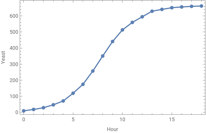
The growth seems to follow a logistic trend. Next, we study the logistic model and estimate its parameters.
Fitting the Logistic Function
Fitting the Logistic Function
The logistic function is :
a/(1+b)
-ct
In[]:=
f1=a/(1+bExp[-ct]);
We fit this model:
In[]:=
bestPars1=FindFit[tY,f1,{a,b,c},t]
Out[]=
{a663.022,b71.5763,c0.546995}
The fitted model is
In[]:=
fit1=f1/.bestPars1
Out[]=
663.022
1+71.5763
-0.546995t
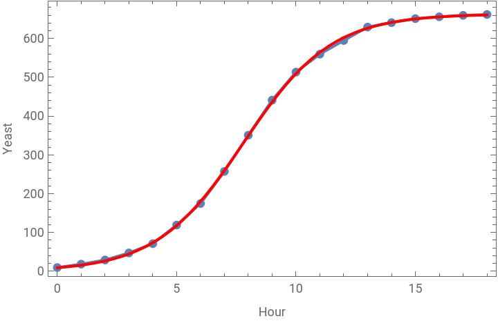
The fit is very good:
In[]:=
Show[ptY,Plot[fit1,{t,0,18},PlotStyle->Red]]
Out[]=
Fitting the Solution of the Logistic DE
Fitting the Solution of the Logistic DE
The logistic function can be seen to be the solution of a logistic DE. Indeed, consider the logistic DE:
In[]:=
eqns={Y'[t]rY[t](M-Y[t]),Y[0]==Y0};
Its solution is as follows:
In[]:=
Y[t]/.DSolve[eqns,Y[t],t]〚1〛
Out[]=
Mrt
M-Y0+Y0
Mrt
This solution can also be written in the form
In[]:=
f2=M1+-1;
M
Y0
-rMt
This model again can be written in the form of f1 above by a simple transformation of the parameters:
In[]:=
Solve[{M==a,M/Y0-1==b,rM==c},{M,Y0,r}]
Out[]=
Ma,Y0,r
a
1+b
c
a
Next, we estimate the parameters of f2:
In[]:=
FindFit[tY,f2,{M,Y0,r},t]
Out[]=
{M393.039,Y09.6,r0.819405}
This is a very bad fit. To get good estimates of the parameters M, Y0, and r, it turns out that we have to give a starting value at least for M or r. From f2, we can see that when t grows, the solution of the DE approaches the value M; from the data, M is thus apparently near to 661.8. We then fit the solution of the logistic differential equation to the data:
In[]:=
bestPars2=FindFit[tY,f2,{{M,661.8},Y0,r},t]
Out[]=
{M663.022,Y09.13552,r0.000825002}
In[]:=
fit2=f2/.bestPars2
Out[]=
663.022
1+71.5763
-0.546995t
This is the same as fit1.
The 2χ Merit Function
The Merit Function
2
χ
It is instructive to see the so-called merit function as a function of some of the unknown parameters. We fix Y0 to be 9.6 and calculate values of the model at the set of the given time instances:
2
χ
In[]:=
pred=f2/.{Y0->9.6,t->Range[0,18]};
Then the residuals are Yeast – pred and the merit function is the inner product of the residuals with itself. However, the figure may be better if we plot the square root of the inner product. This is the same as the Euclidean distance between the data and the predicted values, so that the criterion function to be minimized can be written as
2
χ
In[]:=
crit=EuclideanDistance[Yeast,pred]
Out[]=
0.++++++++++++++++++
2
Abs661.8-
M
1+(-1+0.104167M)
-18Mr
2
Abs659.6-
M
1+(-1+0.104167M)
-17Mr
2
Abs655.9-
M
1+(-1+0.104167M)
-16Mr
2
Abs651.1-
M
1+(-1+0.104167M)
-15Mr
2
Abs640.8-
M
1+(-1+0.104167M)
-14Mr
2
Abs629.4-
M
1+(-1+0.104167M)
-13Mr
2
Abs594.8-
M
1+(-1+0.104167M)
-12Mr
2
Abs559.7-
M
1+(-1+0.104167M)
-11Mr
2
Abs513.3-
M
1+(-1+0.104167M)
-10Mr
2
Abs441.-
M
1+(-1+0.104167M)
-9Mr
2
Abs350.7-
M
1+(-1+0.104167M)
-8Mr
2
Abs257.3-
M
1+(-1+0.104167M)
-7Mr
2
Abs174.6-
M
1+(-1+0.104167M)
-6Mr
2
Abs119.1-
M
1+(-1+0.104167M)
-5Mr
2
Abs71.1-
M
1+(-1+0.104167M)
-4Mr
2
Abs47.2-
M
1+(-1+0.104167M)
-3Mr
2
Abs29.-
M
1+(-1+0.104167M)
-2Mr
2
Abs18.3-
M
1+(-1+0.104167M)
-Mr
We plot this function as a contour plot:
In[]:=
ContourPlot[crit,{M,300,1000},{r,0,0.0015},FrameLabel->{M,r},RotateLabel->False,Contours->15,Epilog->{Red,AbsolutePointSize[6],Point[{M,r}/.bestPars2]}]
Out[]=
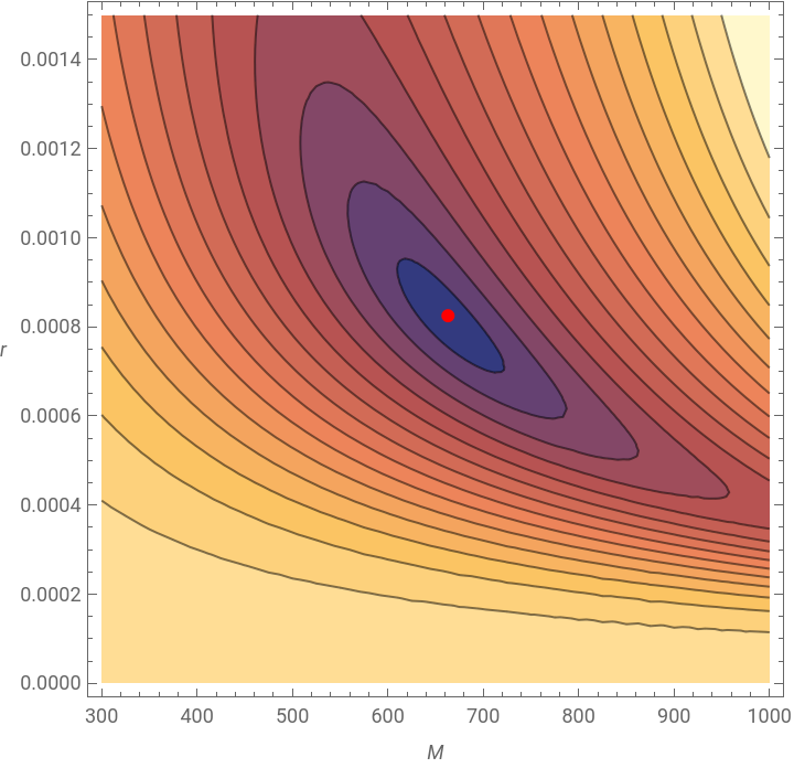
The optimal parameters and are at the red point. The plot gives us confidence that these values of the parameters are the optimal ones.
M
r
Estimates of the parameters can also be found by minimizing the merit function (in this example, we need quite accurate starting values):
Fitting the Logistic DE
Fitting the Logistic DE
Above, we were able to symbolically solve the DE, and this solution could then be estimated. Now we consider the case where we do not have a symbolic solution. First, define the model f3 to be the numerical solution of the equation as a function of the unknown parameters. The result is a parametric function:
We can ask for the solution for given values of the parameters:
We can then fit the parametric function to the data. We give a starting value for r to get a good solution:
This solution is almost the same as bestPars2. Our fitted model is now not an explicit mathematical formula but an interpolating function:
The fit is practically the same as fit1:
Trajectories
Trajectories
It is instructive to see the solution of the logistic DE for a set of initial values. Such a solution set is also called a set of trajectories.
Here, the fitted solution is red.
A direction field is instructive, too. It shows the direction of motion in a given area:
We can combine the two plots:
Example 2: A Predator-Prey Model
Example 2: A Predator-Prey Model
Data
Data
For 26 years, from 1909 through 1934, the yearly numbers of hare and lynx pelts sold to the Hudson Bay Trading Company were as follows (Burghes and Borrie, 1981):
The lynx data for 1914 was lacking; we used the value 14 which is approximately the mean of the surrounding values 19 and 8. A plot is as follows.
For both the hare and lynx data, we can see a cycle of approximately 10 years. Cyclical data is typical for a predator-prey population. When the hare population is low, then soon also the lynx population is low because more than 90% of the diet of the lynx is hare and when there are few hares available, lynx starve rather than eat other species. - As said, the data describes the amounts of sold pelts. Obviously, these amounts reflect the sizes of the hare and lynx populations. So, we may consider the data as describing a predator-pray phenomenon.
We can also plot the pairs of hare and lynx:
The staring point is shown as red. We can see approximately a counterclockwise cycle, typical for a predator-prey system.
For later use, we combine the hare and lynx data pairs into a single list:
Fitting a Predator-Prey Model
Fitting a Predator-Prey Model
In Example 1, we used FindFit to get the fit to the data. Now we do not use FindFit. Instead, we will minimize the Euclidean distance between the data points and points calculated from the solution of the differential equations. To this end, first define the following functions:
Here, f gives the solution of the equations for given parameters, pred calculates predictions from the model, that is, values of the solution at the same time instances as the data, and crit defines the expression to be minimized that is, the square root of the sum of the squares of the differences between the data and the model.
We will minimize crit using FindMinimum. It turns out that the solution to this optimization problem may give very different solutions depending on from where we start the minimization method. Thus, to obtain good starting values for the parameters, we sample the criterion function at a large amount of random points. We then pick the best point of these random points as the starting point to FindMinimum.
For example, here is the first 4-tuple:
We then calculate the value of the criterion function for all of these points:
This calculation took approximately 5 seconds. We plot all the values in the range (0, 500):
The best point is shown as red. Most values are between 200 and 350. We then ask for the best value and the corresponding values of the parameters:
Now we find the optimal values of the parameters by starting the optimization near these values (we need to set the value of a system option):
The minimum value of the criterion is 47.0872, so we were able to halve the minimum value of the random points (97.3364). The estimated equations are
The solution of these equations is
We show the solutions together with the data:
The fits may be reasonable good.
We can illustrate the criterion function by fixing two of the four parameters p, q, P, and Q. In the following plot, we fix P and Q to their optimal values and show the criterion function as a function of p and q:
The optimal point is shown by a red point. The figure shows that the criterion function may well have several local minima, so that finding a good starting point to the optimization may help in finding the global minimum. We can also ask for a contour plot:
Trajectories
Trajectories
The plot of the phase trajectory in the (H, L) plane is as follows:
We show the data, too:
The fitted solution is a closed curve, starting from the big red point and going counterclockwise. Approximately in the time 10.4, the curve closes the first time; recall that, from the data, we saw a cycle of approximately 10 years.
If we sample the solution and show these points, we get an impression about the speed of the development on the curve:
The development is fast at the 4th, 5th, and 6th year of the ten years cycle.
First, compute solutions of the equations such that, at time 0, H is 40 and L gets values from 0.5 to 3.5 in steps of 0.5:
A direction field tells the direction to which the trajectory goes from a set of points:
We combine the trajectory plot, the vector plot, and the plot of the nullclines together with the trajectory of the original equation:
Equilibrium Points
Equilibrium Points
The last figure above shows that the cross point of the nullclines is a so-called center. The result can also be verified mathematically. To this end, the equilibrium points are as follows:
To investigate the nature of the equilibrium points, first calculate the Jacobian of the derivatives:
Here are the equilibrium points and eigenvalues of the Jacobian at the equilibrium points, by using the estimated parameters:
From the theory of dynamical systems we know that an equilibrium point is
Example 3: A Chemical Model
Example 3: A Chemical Model
Data
Data
In Moura (2016), a kinetic model is considered. Variables V, X, Y, and Z are concentrations of four reactants. These variables were measured at 12 times, in addition to the initial values at time 0:
The measurements were as follows:
To plot the data, we add the time instances:
It may also be instructive to see how pairs of variables evolve. The starting point is red:
For later use, we combine the measurements of the variables into a single list:
Numerical solution
Numerical solution
The linear system of differential equations in Moura (2016) is as follows:
We also define the time interval of the data:
Later, we will see that we can solve this system symbolically with DSolve or with the aid of the matrix exponential function. However, to get estimates of the parameters, the symbolic solution is useless because it is extremely complicated. Thus, it is better to get estimates of the parameters with our numeric method we have used in Examples 2 and 3. Recall that the numerical solution of the DE system is expressed in terms of interpolation functions. However, we can get the solution in terms of mathematical expressions, too, by substituting the estimates of the parameters into the symbolic solution.
So, here we estimate the parameters with our numeric method. As in Examples 2 and 3, we will minimize the Euclidean distance between the data points and points calculated from the solution of the differential equations. To this end, first define the following functions:
Note that when the numerical solution is tabulated in pred, we have to use the unevenly spaced time instances that were earlier stored in tt.
We then calculate the value of the criterion function for all of these points:
The computation took approximately 4 seconds. Here are the values of the criterion function:
We search the optimum values of the parameters by starting near to the best random values:
The best model is
The solution of these equations is
We compare the data and the curves given by the DYs:
The fitted curves very well follow the data and so we can say that the estimated model is good.
We can again illustrate the criterion function by fixing two of the four parameters a, b, c, d, e, and f. In the following plot, we show the criterion function as a function of a and b; all other parameters are fixed to their optimal values (note that the function is clipped at one corner).
The optimal point is shown by a red point. The criterion function seems to be quite easy to minimize. A contour plot is as follows (note again that the function is clipped at the lower left corner):
Trajectories
Trajectories
Two-dimensional trajectories are as follows:
Here are the three-dimensional trajectories:
Symbolic solution
Symbolic solution
As the differential equations of the kinetic model are linear, we are able to solve the system symbolically, too:
However, the symbolic solution is useful together with the numerical solution. Recall that the best values of the parameters from the numerical solution were as follows:
Now we can calculate the symbolic solution by using these numerical values for the parameters. This solution is quite simple:
We plot the solution:
The difference is practically zero, so that the solutions are practically the same.
We can also substitute the best parameters into the differential equations:
Then we can solve these equations:
The solution is the same as in fit2.
References
References
Burghes, D. N., and M. S. Borrie (1981), Modelling with Differential Equations, Horwood, Chichester, UK.
Laska, T. (2019), Estimating parameters on system of differential equations, https://mathematica.stackexchange.com/questions/197903/estimating-parameters-on-system-of-differential-equations.
Moura, I. (2016), Parameter estimation for a system of differential equations, https://se.mathworks.com/matlabcentral/answers/314965-parameter-estimation-for-a-system-of-differential-equations.
Pearl, R. (1927), The growth of populations, Quarterly Review of Biology 2(4), 532-548, https://www.journals.uchicago.edu/doi/epdf/10.1086/394288.
Ramsay, J. O., G. Hooker, D. Cambell, and J. Cao (2007), Parameter estimation for differential equations: a generalized smoothing approach, Journal of the Royal Statistical Society, Series B, Statistical Methodology, 69(5), 741-796, https://rss.onlinelibrary.wiley.com/doi/full/10.1111/j.1467-9868.2007.00610.x.
Ruskeepää, H. (2009), Mathematica Navigator: Mathematics, Graphics, and Statistics, 3rd Ed., Academic Press, Cambridge.
CITE THIS NOTEBOOK
CITE THIS NOTEBOOK
Estimation of parameters in differential equation models
by Heikki Ruskeepää
Wolfram Community, STAFF PICKS, November 13, 2023
https://community.wolfram.com/groups/-/m/t/3064641
by Heikki Ruskeepää
Wolfram Community, STAFF PICKS, November 13, 2023
https://community.wolfram.com/groups/-/m/t/3064641