Particle tracks in bubble chamber
By Syed Waqar Ahmed
National University of Computer and Emerging Sciences, Karachi, Pakistan
By Syed Waqar Ahmed
National University of Computer and Emerging Sciences, Karachi, Pakistan
We intend to study the images of spiral tracks left behind by charged particles inside a bubble chamber. We are particularly interested in the consistent spiral forms and describe a pathway for the students to study these spirals. We have extracted the track decay information from the images.
Bubble Chamber in Classrooms
Bubble Chamber in Classrooms
Overview
Overview
The Bubble chambers were one of the pioneer experiments in particle tracking, studying and discovering the new subatomic particles. These apparatus allowed the observation of particle interactions and behavior under the effects of constant magnetic field. The students are taught the Lorentz force on charged particles in college without much experimental evidence; However, enough data has been collected about the tracks formed by the charged particles that can be used in the classroom as simulations or computational methodology to match and study the particle behavior as observed in the experiments.
This projects aims to lay a pathway for students to study the particle track from the images using image data collection, processing and finding useful information from the 2D geometry.
Issues with Extracting Information from Images
Issues with Extracting Information from Images
The construction of a bubble chamber requires a volume of diffused gas that can be ionized and clusters around the energetic particle passing though the volume. In order to study the 2D picture, the particle must also travel in this 2D plane as well. Therefore, we will proceed with the approach of finding pictures where the tracks do not show a drift or skew in the spiral form—spiral form that we will call a consistent spiral form.
Commonly available image data is lacking information about the magnitude and direction of the magnetic field strength, , orientation and size of the chamber and scale of the image. The information of gas type and density is also important and missing.
B
Why Spiral Trajectories?
Why Spiral Trajectories?
The charged particle enters the Bubble chamber with some kinetic energy. Under the presence of a constant perpendicular magnetic field, a charged particle curves its path due to the Lorentz force. The gas inside the chamber acts as a viscous medium and the collisions with these gas particles make the particles lose energy; for decreasing velocities, the curve shrinks and forms continuous spirals. Viscosity will be introduced into the differential equations to the simulate bubble chamber environment.
Differential Equations
Differential Equations
We construct the differential equations and the solution for Lorentz force.
Define the position vector:
In[]:=
Define the magnetic field vector:
In[]:=
In[]:=
eqns=Threadmq
2
∂
∂
2
t
∂
∂t
Out[]=
{m(t)q(t),m(t)(-q)(t),True}
′′
x
′
y
′′
y
′
x
Introduce a viscosity term, γ, into the differential equation:
eqnswithvisc=Most@Threadmq-γ
2
∂
∂
2
t
∂
∂t
∂
∂t
Out[]=
{m(t)q(t)-γ(t),m(t)(-q)(t)-γ(t)}
′′
x
′
y
′
x
′′
y
′
x
′
y
Solve the differential equation:
In[]:=
xysol=First@DSolve[eqnswithvisc,{x,y},t]
Out[]=
x{t}m-γcos+qsin+γ++mq-γsin-qcos++,y{t}m-γcos+qsin+γ+-mq-γsin-qcos++
c
2
-
γt
m
qt
m
qt
m
γt
m
2
γ
2
2
q
c
4
-
γt
m
γt
m
qt
m
qt
m
2
γ
2
2
q
c
1
c
4
-
γt
m
qt
m
qt
m
γt
m
2
γ
2
2
q
c
2
-
γt
m
γt
m
qt
m
qt
m
2
γ
2
2
q
c
3
Define the initial conditions:
In[]:=
ICs={x(0)0,y(0),(0)0,(0)};
0
′
x
′
y
0
Solve the differential equation:
In[]:=
solnwithICs=First@DSolve[Join[eqnswithvisc,ICs],{x,y},t]
Out[]=
x{t}+,y{t}-γmcos+mqsin++γm+
mq-γsin-qcos
0
-
γt
m
γt
m
qt
m
qt
m
2
γ
2
2
q
0
-
γt
m
2
2
q
γt
m
qt
m
qt
m
2
γ
γt
m
γt
m
2
γ
2
2
q
Using the solutions, students can observe the impact of each parameter on the curve. This idea can help build intuition of the types of tracks and spiral one observes in the images.
Change the parameters in the differential equation to see how the spiral changes:
Out[]=


The above solutions can be used with specific values of the parameters to approximate the path.
Extracting data and finding functions
Extracting data and finding functions
In order to study the real images without experimental information we will try to utilize the geometric information. Notice that for the following images, the time information is also missing.
Step 1: Coordinate tracking
Step 1: Coordinate tracking
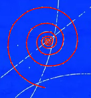
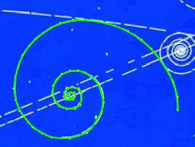
With the help of image manipulation panel in wolfram, students will trace the points on curve that will serve as the data. Notice that the larger number of points are required for the smaller curvature in order to fit the spline function accurately.
Step 2: Generating a spline function
Step 2: Generating a spline function
image[1]=
;
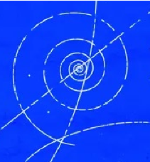
Extract coordinate data from the image:
In[]:=
imagedata[1]=;
Fit a spline function to the data:
In[]:=
splinea=BSplineFunction[imagedata[1]]
Out[]=
BSplineFunction


Display the image and spline fit together:
In[]:=
Show[image[1],ListPlot[imagedata[1],PlotStyleYellow],ParametricPlot[splinea[x],{x,0,1},PlotStyle->Red]]
Step 3: Normalizing the data and plotting
Step 3: Normalizing the data and plotting
ra=Table[Norm[splinea[0]-splinea[p]],{p,0,1,0.01}];
nra=N@ra/Last[ra];
ListPlot[{Reverse[nra],Reverse[nrb],Reverse[nrc]},PlotStyle->{Red,Orange,Green},AxesLabel{"spline segments","Normalized Radius"}]
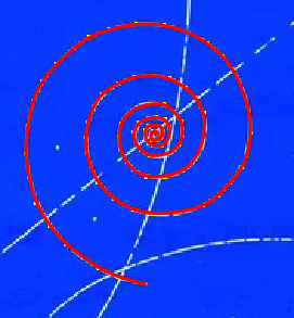
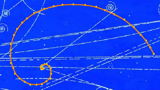
Below, we plot radius as a function of spline segments for the three spirals in the test image.
Out[]=
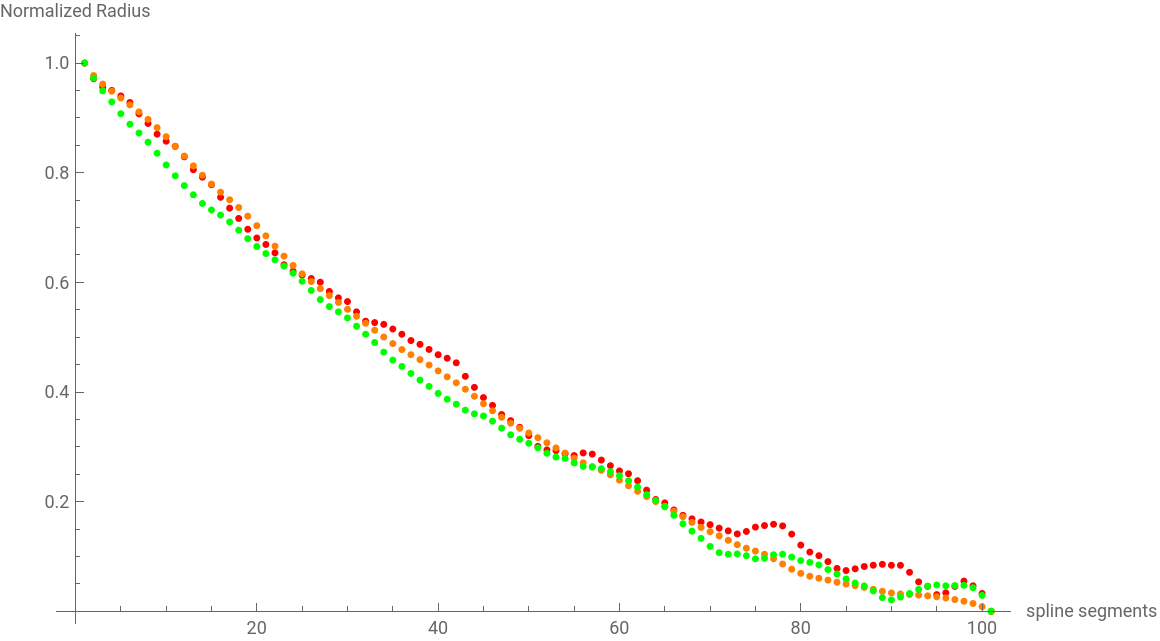
It is evident that the different spirals are displaying similar information in the above plot. We can therefor utilize this information as the necessary information of the spiral.
Concluding remarks
Concluding remarks
The above procedure describes a computational analyses laying the pathway for the students to start learning and extracting information about the curve. Using an image of particle tracks without other information, we have analyzed the geometric data to approximate the radius reduction factor.
This project can be improved by including the relativistic effects in for the particles and by using machine learning to auto detect the spiral tracks.
Future Work
Future Work
Keywords
Keywords
◼
Particle physics
◼
Bubble chamber
◼
Spirals
◼
Lorentz force
Acknowledgment
Acknowledgment
Thanks for the guidance, encouragement and all the help to my mentors, Paul Abbott and Craig Carter!