Abstract: Shown below is an exploration of feature based methods for estimating camera position in relation to a 3D object. Using only synthetic data, three potential approaches are investigated with varying levels of complexity and generalizability. First, a simple method using standard computational photography techniques and a notion of weighted nearest neighbor . Second, a convolutional neural network encoder that directly predicts camera position from a given test image. Lastly, a transfer learning based approach where networks trained on real world object recognition and segmentation tasks are used as feature detectors for predicting camera position. A discussion concerning the merits and limitations of each method is presented and a promising research direction is proposed.
Introduction:
Introduction:
Estimating the orientation of a known object in a scene is a well studied problem in computer vision with many applications in fields such as robotic manipulation, motion tracking and general scene understanding . While many approaches exist, most can be thought of as belonging to one of two core methodologies.
Direct Point Correspondence: A set of methods were a direct mapping between points on a 3D model and points in a 2D image is known a priori. With this information given at the outset there exist both iterative and closed form solutions to the problem. While this method can be very accurate under the right conditions, creating an environment were all the required information is known is a non-trivial task. More information on one such method can be found here: Perspective-n-Point.
Feature Based Correspondence: A set of methods that extracts features from a 2D image which can then be related to known information about a 3D model. Features can be extracted by a number of methods including but not limited to, image key point detection and neural network embeddings. This approach does have the draw back of potentially being more computationally expensive, either requiring large amounts of training data and/or expensive computation at inference time. Despite these limitations, feature based methods have become the focus of many modern research efforts due to a reduced dependence on a priori information and their general flexibility.
For the remainder of this post the focus will be exclusively on feature based methods as I believe they are better suited to a wider array of potential use cases.
1. The Easy Way : Brute Force
1. The Easy Way : Brute Force
One very direct method to achieve this goal would be to take a large number of images of an object from many different angles and save them. When a test image comes in, compare the test image with the saved images via image correspondence methods (e.g. ORB, SURF, etc.), and return the known angle of the closest match.
1.1 The object:
◼
This function will get an object ready to use for our purposes.
In[]:=
getBaseGeometry[model_String,view_List:{0,-2,0}]:=Graphics3D[ExampleData[{"Geometry3D",model}][[1]],ViewPoint->view,Boxed->False,Lighting->"Accent"];
◼
Now lets select one of the available objects
In[]:=
availableObjects=#[[2]]&/@ExampleData["Geometry3D"]rabbit=getBaseGeometry["StanfordBunny",{1,-2,0}]
Out[]=
{BassGuitar,Beethoven,CastleWall,Cone,Cow,Deimos,Galleon,HammerheadShark,Horse,KleinBottle,MoebiusStrip,Phobos,PottedPlant,Seashell,SedanCar,SpaceShuttle,StanfordBunny,Torus,Tree,Triceratops,Tugboat,UtahTeapot,UtahVWBug,Vase,VikingLander,Wrench,Zeppelin}
Out[]=
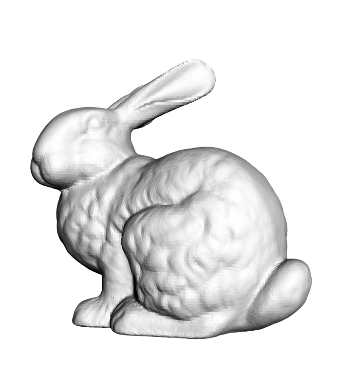
◼
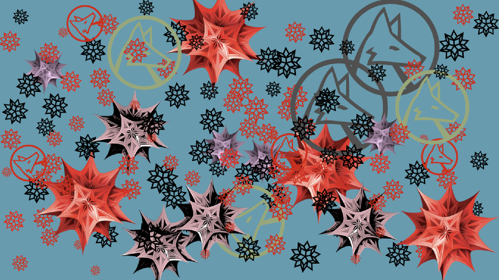
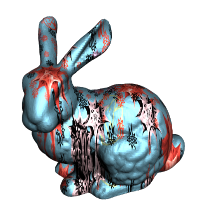
Image correspondence methods will perform better with some variation in texture, let’s wrap the geometry with an image texture. This function takes a geometry and wraps it in a given image.
In[]:=
getWrappedGeometry[model_String,texture_Image,view_List:{0,-2,0}]:=Graphics3D[{Specularity[White,10],RegionPlot3D[DiscretizeGraphics@ExampleData[{"Geometry3D",model}],PlotStyle->Directive[Texture[texture]],Boxed->False][[1]]},Boxed->False,ViewPoint->view,Lighting->"Accent"]
◼
Select a texture image and wrap the geometry.
In[]:=
textureImage=
;wrappedRabbit=getWrappedGeometry["StanfordBunny",textureImage,{1,-2,0}]
Out[]=
1.2 Multiple views of the object:
In[]:=
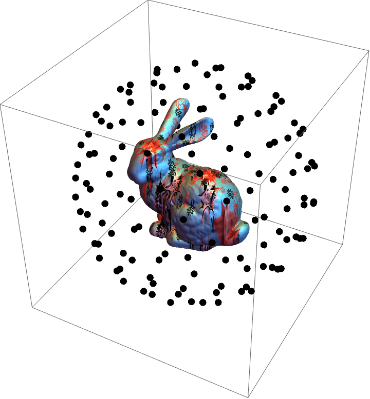
Graphics3D[{PointSize[Large],Point[({-.02,0,.1}+#)&/@(0.15*SpherePoints[144])],wrappedRabbit〚1〛},BoxedTrue]
Out[]=
◼
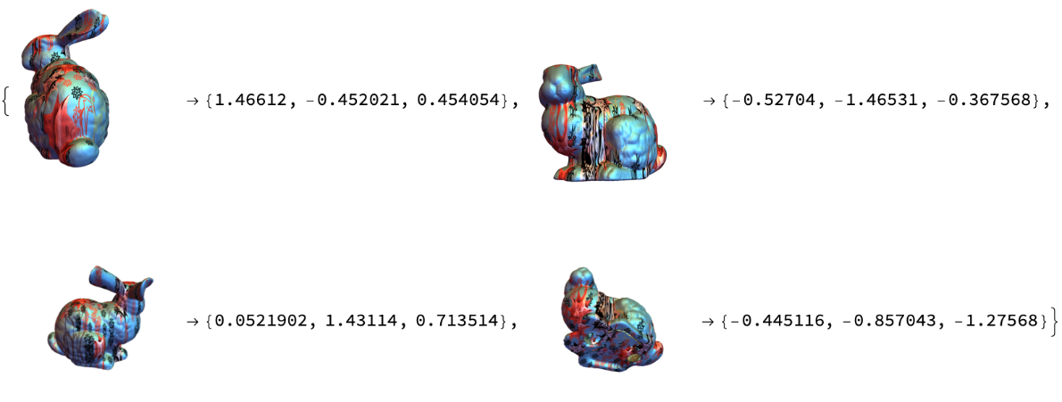
This function will collect the data from a specified number of evenly spaced view points.
In[]:=
createReferenceData[geometry_,n_Integer,imgWidth_]:=(viewPoints=1.6*SpherePoints[n];createdData=(ImageResize[Image[Graphics3D[First@geometry,ViewPoint#,BoxedFalse]],imgWidth]#)&/@viewPoints;Return[{viewPoints,createdData}]);
In[]:=
collectedRabbitData=createReferenceData[wrappedRabbit,72,512];RandomSample[collectedRabbitData〚2〛,4]
Out[]=
1.3Estimateanovelviewusingimagecorrespondence
◼
This function estimates the view by considering the raw image correspondence results and performs a weighted average over the k highest ranking views. The interpolation step is an attempt to gain finer resolution than is available purely through the data sample.
In[]:=
estimateView[results_,k_]:=(refViews=Keys[results〚1〛];(*Findtheindexofthebestmatchingsinglepointforeachtestimage.*)bestMatch=Table[TakeLargest[Values[results〚i〛]"Index",1],{i,1,Length[results]}];(*Findthecameralocationforeachbestmatchforeachtestimage.*)bestLocs=Table[results〚i〛〚bestMatch〚i〛〛〚1〛〚1〛,{i,1,Length[bestMatch]}];(*Findtheanglebetweenthebestcamerapositionforeachtestimagetotheotherreferencelocations.Thisisdonesothatwecanconsiderthestrengthofneighboringpointstorefinethecameraposition.*)angleToBest=Table[(VectorAngle[bestLocs〚i〛,#])&/@refViews,{i,1,Length[bestLocs]}];(*Getatheindicesforneighborhoodofpointstoconsiderforeachtestimage*)consideredIndexs=Table[TakeSmallest[angleToBest〚i〛"Index",k],{i,1,Length[angleToBest]}];resultPositions=Table[(results〚1〛〚#〛〚1〛)&/@consideredIndexs〚i〛,{i,1,Length[consideredIndexs]}];resultWeights=Table[N[Normalize[(results〚i〛〚#〛〚2〛)&/@consideredIndexs〚i〛,Total[#,∞]&]],{i,1,Length[consideredIndexs]}];viewEst=Table[Mean[WeightedData[resultPositions〚i〛,resultWeights〚i〛]],{i,1,Length[resultPositions]}];Return[viewEst];)
◼
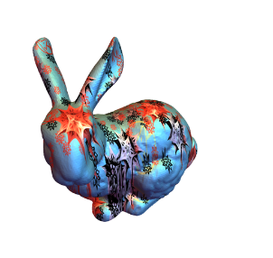
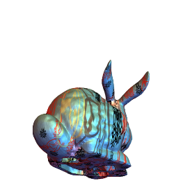
Let’s test it out. Here are some test images along with the correct views.
In[]:=
testViews=
->{-0.4,-1.05,1.102},
{1.01,0.85,-0.886};rawResults=Table[(#〚2〛->Length[ImageCorrespondingPoints[testViews〚i〛〚1〛,#〚1〛]〚1〛])&/@collectedRabbitData〚2〛,{i,1,Length[testViews]}];viewEstimates=estimateView[rawResults,4]
Out[]=
{{-0.529295,-0.970268,1.1033},{1.04159,0.814216,-0.838509}}
◼
Evaluating the accuracy of the results measured in degrees.
Image correspondence methods are sensitive to everything visible in the photograph. This means the resolution of the image and the density of sampling points will have a significant impact on the accuracy of the results. Below is a more robust evaluation of trade-offs between these factors.
The legend is read as follows: 144v720 = 144 sampling points at an image width of 720 pixels
The legend is read as follows: 144v720 = 144 sampling points at an image width of 720 pixels
The image correspondence method does work, but only in very controlled conditions. What if someone wanted a different texture on the object? How about a background that is not simply flat white? How about a more difficult object with fewer distinguishing geometric features? Every permutation that might change the output of the selected image correspondence method would need to be sampled at a high enough density to allow for a meaningful measurement. This is especially problematic since we need to do the core computation of finding image correspondences for every image in the data sample for each new test image.
2. Learning Based Approach : Neural Network Features
2. Learning Based Approach : Neural Network Features
If we would like to be able to make predictions about the orientation of an object regardless of its background or texture we need a way of paying attention to only the relevant factors. By collecting a dataset in which a single item with a single orientation is associated it with a variety of textures, backgrounds, and positions we give a network the opportunity to learn other factors relevant to orientation estimation.
2.1 Data... a lot of it:
If we want the networks to be invariant to certain changes in the image we must demonstrate the required variability through the data. We will need:
◼
A variety of object textures
◼
A variety of background textures
◼
A more difficult geometry (just for fun)
◼
Now we need a function to mix them all together along with some random shifts in position.
◼
Create some data
2.2 Direct Prediction Convolutional Encoder:
2.2 Direct Prediction Convolutional Encoder:
◼
Build a convolutional encoder network and train it from scratch.
*NOTE* Below is only a sample of what the training code would look like. To properly train this model a much larger and randomized training sample is required
◼
Evaluate the encoder on some test data
The trained network used here is loaded from a local resource
At first glance this looks great. Not only does the encoder predict with a higher accuracy than the brute force method, it does so in the presence of multiple object/background textures and shifts in the position of the object. How general is it though? Let’s look at some real images.
Not great. Pretty bad actually. It looks like while the encoder model has become robust to specific types of variation present in the training set, it does not generalize well to natural images. Can we do better?
2.3 Direct Prediction Transfer Learning:
Rather than training our network from scratch perhaps we can leverage training that has already been performed on real world data. For this next set of experiments two pretrained networks are selected that have similar objects (guitars in this case) present in their training sets. The selected networks for this sections are MobileNet v2 and Ademxapp Model A1 trained on ImageNet and ADE20K respectively. The remainder of this section will focus on the adaptation of MobileNet v2 as both are set up in a similar way and the trained networks show similar results.
◼
Perform network surgery on MobileNetv2 to extract the desired layers. Add the required layers to directly predict orientation from the low level features
*NOTE* Below is only a sample of what the training code would look like. To properly train this model a much larger and randomized training sample is required. Additionally, in this instance images with a square dimension of 224 would also be required.
◼
Evaluate the trained MobileNet v2 transfer network on some test data
The trained network used here is loaded from a local resource
Again these results are promising. Transfer learning does not perform quite as well as the encoder network on purely synthetic data however it is comparable with the brute force method, and maintains robustness to the added variability like the encoder does. What about real world images?
A surprising result. Keep in mind the original MobileNet v2 architecture was not trained to predict object orientation. In addition, no real world data was used in the transfer learning training process to obtain the results you see here.
3. Discussion and Next Steps
3. Discussion and Next Steps
◼
Most of the key results in this post could have perhaps been predicted at the outset.
◼
The brute force method while accurate is extremely context specific and computationally expensive.
◼
The network trained from scratch only on synthetic data was able to handle the variation present in the training data and yielded extremely accurate results but was unable to generalize to real world data.
◼
One result is surprising and perhaps suggests a promising avenue for future research.
◼
The transfer learning approaches were able to learn to predict object orientation with a high degree of accuracy while simultaneously remaining robust to some (though not all) real world data. It is worth noting again that no real world training data was used to achieve this result. Future research may dig deeper into this result to determine answers to the following:
1
.Is the object category required to be in the original real world training set (as was the case here) for this method to be effective?
2
.Can additional benefits be gained by adding synthetic data to the initial object classification or segmentation training sets?
3
.What other objectives can be trained in this way. For example can you train a segmentation model on only synthetic data if you have an object classifier trained on real world data pertaining to the segmentation target.