This notebook introduces planetary resonance through orbital variables, a Fourier expansion of the interaction Hamiltonian, and integer relations among angular rates. A constant-rate approximation illustrates how the interaction phase controls harmonic cancellation and accumulation. Mean-motion, secular, and spin–orbit resonances are presented through concise definitions and examples. Wolfram Language animations visualize the accumulation of individual harmonics, with the corresponding code provided in the Appendix. This project constitutes one of the lectures for Planetary Theory I in the preliminary PhD program in Mathematical Astronomy, Department of Astronomy, Space Science and Meteorology, Faculty of Science, Cairo University, under the supervision of Professor Walid Rahoma.
1 Orbital Variables
1 Orbital Variables
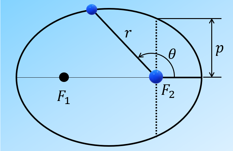
The Newtonian two-body problem describes the motion of two point masses interacting only through their mutual gravitational attraction. Let be the distance between the masses. For a noncircular elliptical orbit, the true anomaly is measured at the occupied focus from periapsis to the relative position vector in the direction of motion, as illustrated in Fig. 1.
r
θ
F
2
F
2
r
θ
p
The trajectory is expressed as:
r=,
p
1+ecosθ
(
1
)where is the semilatus rectum, is the semimajor axis, and is the eccentricity. Elliptical motion is considered here, with . The orbital geometry is specified by Eq. (1), but the position at a given time is not obtained directly from it. To establish the connection between time and position, two additional angular variables are introduced: the mean anomaly and the eccentric anomaly . The mean anomaly is defined as a uniformly increasing orbital phase:
p=a(1−)
2
e
a
e
0≤e<1
M
E
M=n(t−τ),
(
2
)where is time, is the time of periapsis passage, and is the mean motion. For an unperturbed two-body orbit, the mean motion is given by:
t
τ
n
n=,
μ
3
a
(
3
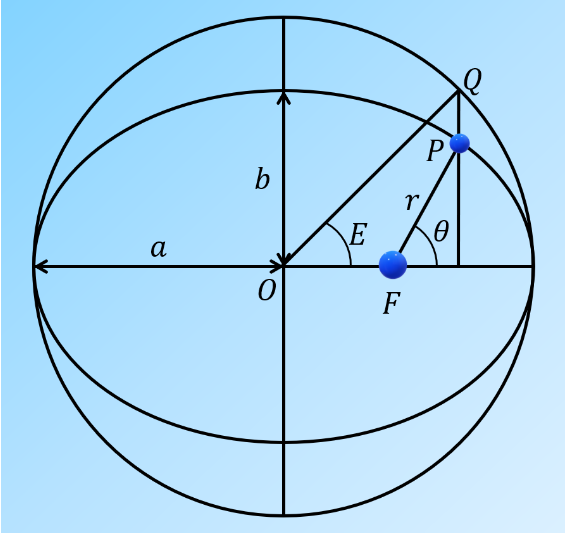
)where is the gravitational parameter, is the gravitational constant, and and are the two masses. The orbital period is related to the mean motion through . Although is expressed as an angle, the actual direction of the body from the focus is specified by . To connect this time-dependent phase to the orbital geometry, an auxiliary circle of radius is drawn about the center of the ellipse, as illustrated in Fig. 2. From the orbital position , a line perpendicular to the major axis is extended to the corresponding point on the circle. The eccentric anomaly is measured at from the periapsis direction to .
μ=G(+m)
m
0
G
m
0
m
T
n=2π/T
M
θ
a
O
P
Q
E
O
OQ
E
a
b
θ
The mean and eccentric anomalies are related by Kepler’s equation:
M=E−esinE.
(
4
)Once has been obtained from , the orbital distance is calculated from:
E
M
r=a(1−ecosE).
(
5
)The true anomaly is then obtained using:
tan=tan.
θ
2
1+e
1−e
E
2
(
6
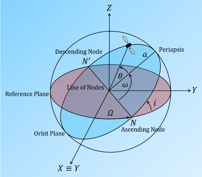
)Thus, with the appropriate angular quadrant retained, the position at a given time is obtained through the sequence . The orientation of this planar orbit in three-dimensional space must also be specified. A reference plane and a fixed reference direction are adopted, as illustrated in Fig. 3. The intersection of the orbital and reference planes defines the line of nodes. The ascending node is identified where the body crosses the reference plane toward its positive normal.
t→M→E→(r,θ)
X≡Υ
i
Ω
ω
θ
The orbital size and shape are specified by and , respectively. The inclination is the angle between the orbital angular-momentum vector and the positive normal to the reference plane. The longitude of the ascending node is measured in the reference plane from the reference direction to the ascending node . The argument of periapsis is measured in the orbital plane from the ascending node to periapsis in the direction of motion. A complete set of orbital elements therefore consists of , and an orbital phase at a specified epoch. The mean anomaly is adopted as the sixth element here. An equivalent phase specification may be provided by or by the periapsis-passage time . The angular geometry shown in Fig. 3 is further illustrated in the accompanying Demonstration, Geometry of Keplerian Orbital Parameters, in which , and can be varied interactively.
a
e
i
Ω
X≡Υ
N
ω
N
a,e,i,Ω,ω
M
θ
τ
i,Ω,ω
θ
Observe the variation of the four angular parameters () and examine their effect on the spatial orientation of the orbit and the position of the satellite:
i,Ω,ω,θ
In[]:=
ResourceObject["Demonstration: Geometry of Keplerian Orbital Parameters"]
Out[]=
ResourceObject


ResourceData["Demonstration: Geometry of Keplerian Orbital Parameters"]
Out[]=


For the prograde configurations considered here, additional angular variables are constructed from the orbital elements. The longitude of periapsis is defined by:
ϖ
ϖ=Ω+ω.
(
7
)The mean longitude, , is defined by:
λ
λ=ϖ+M.
(
8
)For inclined orbits, and are measured in different planes. The longitude of periapsis is a composite angle rather than the projected geometric direction of periapsis. The angular rates used below are:
Ω
ω
ϖ
◼
M
◼
n
n=
M
◼
θ
◼
g=
ϖ
◼
s=
Ω
◼
ω
◼
λ
◼
ψ
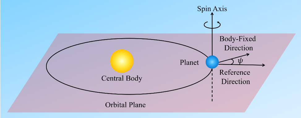
The dot denotes a time derivative. The spin angle describes the rotation of the body about its own axis (spin). As illustrated in Fig. 4, is measured from a fixed reference direction to a direction fixed in the body. In the planar model considered here, the spin axis is assumed to be perpendicular to the orbital plane, and both directions used to measure lie in that plane.
ψ
ψ
ψ
ψ
2 Resonance Mechanism
2 Resonance Mechanism
Display the harmonic accumulation animations with nonzero and zero final accumulations, respectively:
3 Resonance Types
3 Resonance Types
References
References
[2] Lee, T., Leok, M., and McClamroch, N. H. (2007). Lie group variational integrators for the full body problem. Computer Methods in Applied Mechanics and Engineering, 196, 2907–2924. DOI: 10.1016/j.cma.2007.01.017.
[3] Gkolias, I., Celletti, A., Efthymiopoulos, C., and Pucacco, G. (2016). The theory of secondary resonances in the spin–orbit problem. Monthly Notices of the Royal Astronomical Society, 459, 1327–1339. DOI: 10.1093/mnras/stw752.
[4] Forgács-Dajka, E., Sándor, Zs., and Érdi, B. (2018). A fast method to identify mean motion resonances. Monthly Notices of the Royal Astronomical Society, 477, 3383–3389. DOI: 10.1093/mnras/sty641.
[5] Barnes, R., and Greenberg, R. (2006). Extrasolar planetary systems near a secular separatrix. ApJ, 638, 478–487. DOI: 10.1086/498736.
[6] Petrovich, C., Wu, Y., and Ali-Dib, M. (2019). Secular transport during disk dispersal: the case of Kepler-419. AJ, 157, 5. DOI: 10.3847/1538-3881/aaeed9.
[7] Fejoz, J., and Guardia, M. (2023). A remark on the onset of resonance overlap. arXiv: 2308.15222.