An Agile Guide to The Wolfram Language
An Agile Guide to The Wolfram Language
Computational Thinking Modules

JulianJacklin
This guide offers technical knowledge, skills, and tips supplementary to the Computational Thinking Modules. As such, educators, students, and the like may refer to this single guide for any of the following:
- The basics of Wolfram Language
- Mathematical background for advanced concepts.
- Common technical errors and their solutions.
- Domain-specific tools in Wolfram Language.
This is not a comprehensive guide to the Wolfram Language, but instead an agile one which aims to offer timely, pointed support. The Wolfram Language and its associated platforms cover a vast landscape of topics and technologies—this guide tightens the scope around just what is needed for completion and facilitation of the Computational Thinking Modules.
- The basics of Wolfram Language
- Mathematical background for advanced concepts.
- Common technical errors and their solutions.
- Domain-specific tools in Wolfram Language.
This is not a comprehensive guide to the Wolfram Language, but instead an agile one which aims to offer timely, pointed support. The Wolfram Language and its associated platforms cover a vast landscape of topics and technologies—this guide tightens the scope around just what is needed for completion and facilitation of the Computational Thinking Modules.
Introduction
Introduction
What is the Wolfram Language
What is the Wolfram Language
Wolfram Language (WL) is a symbolic language—meaning a language that uses symbols to convey complex ideas—that is designed to help people across disciplines create power programs quickly, and with ease. Programs are sets of directions we give to a computer in order for it to complete the tasks we want it to. Wolfram Language makes this process intuitive by building in as much knowledge—about the world—into the language as possible. By integrating high-level forms—like Image, GeoPolygon or Molecule—along with advanced superfunctions—such as ImageIdentify or ApplyReaction—Wolfram Language makes it possible to quickly express complex ideas in computational form.
In short, you can do a lot using Wolfram Language, often by using plain English.
In short, you can do a lot using Wolfram Language, often by using plain English.
Getting Set Up
Getting Set Up
To use the Wolfram Language you must first have a Wolfram ID. Once this is created, you will have access to Wolfram cloud and can create a new notebook from your browser.
How to Use the Wolfram Language
How to Use the Wolfram Language
As with natural languages (languages humans use to communicate with other humans, like English or Spanish), we need a way to use them. In English, for instance, I can write my ideas on a piece of paper, or say them our loud. To successfully use the Wolfram Language you must write it in a notebook, a digital environment where you can run your code. Please follow the following link for a video tutorial on using notebooks in the WL: cloud (browser). This is step 0 to creating really cool things really quickly.
This notebook is an amazing introduction to said cool things, and can be used once you have a Wolfram ID.
This notebook is an amazing introduction to said cool things, and can be used once you have a Wolfram ID.
Wolfram Basics
Wolfram Basics
Getting Started
Getting Started
To get started using the Wolfram Language, please refer to this free tutorial, containing both text and video resources(Recommended reading includes chapters 1-4, 7, 10-11). This guide does not include a tutorial, but instead a reference for common actions in the language—especially for those that appear often in the CT Modules.
Quick Tips
Quick Tips
Below are some quick reminders and shorthand notation for programming in WL:
@ — prefix form for function application: f@x is the same as f[x]. So Sqrt@16 = 4
/@ — Map shorthand: f /@ list applies f to every element, same as Map[f, list]. So Sqrt/@{9,16,25} = {3,4,5}
; — suppresses output of a line (ensuring code doesn't appear as an output if you don't want it to)
?FunctionName (or ??FunctionName for more detail) pulls up quick documentation right in the notebook (faster than searching online)
Square brackets [ ] are always for function arguments, curly braces { } are always for lists, parentheses ( ) are just grouping — Wolfram is strict about this, unlike math notation where they're often interchangeable
N[...] forces a numeric (decimal) result — helpful since Wolfram keeps things exact/symbolic by default (1/3 stays a fraction until you ask otherwise)
@ — prefix form for function application: f@x is the same as f[x]. So Sqrt@16 = 4
/@ — Map shorthand: f /@ list applies f to every element, same as Map[f, list]. So Sqrt/@{9,16,25} = {3,4,5}
; — suppresses output of a line (ensuring code doesn't appear as an output if you don't want it to)
?FunctionName (or ??FunctionName for more detail) pulls up quick documentation right in the notebook (faster than searching online)
Square brackets [ ] are always for function arguments, curly braces { } are always for lists, parentheses ( ) are just grouping — Wolfram is strict about this, unlike math notation where they're often interchangeable
N[...] forces a numeric (decimal) result — helpful since Wolfram keeps things exact/symbolic by default (1/3 stays a fraction until you ask otherwise)
Functions
Functions
More than most other things, functions will appear frequently in WL. Just as we first learn about them in math, functions are objects that take in an input, and give back an output. Some common functions and their uses are as follows:
- Tabular
Makes yours data into a useable table with columns and rows.
- Tabular
Makes yours data into a useable table with columns and rows.
In[]:=
Tabular[{{1,2,3},{4,5,6}}]
Out[]=
Tabular


In[]:=
Tabular[{{1}}]
Out[]=
Tabular
In[]:=
Tabular[{<|"cookies"3,"cakes"6,"muffins"8|>}]
Out[]=
Tabular
- Dimensions and ColumnKeys
Takes in a data object, like the ones above, and returns the dimensions and column names respectively.
Takes in a data object, like the ones above, and returns the dimensions and column names respectively.
In[]:=
MyPastryShop=Tabular[{<|"cookies"3,"cakes"6,"muffins"8|>}]
Out[]=
Tabular
In[]:=
Dimensions[MyPastryShop]
Out[]=
{1,3}
In[]:=
ColumnKeys[MyPastryShop]
Out[]=
{cookies,cakes,muffins}
- GroupBy
Takes a list and sorts its elements into "buckets" based on a rule you give it — like sorting a pile of mixed fruit into baskets by color.
Takes a list and sorts its elements into "buckets" based on a rule you give it — like sorting a pile of mixed fruit into baskets by color.
In[]:=
MyFruit=Tabular[{<|"name""banana","color""yellow"|>,<|"name""apple","color""red"|>,<|"name""watermelon","color""green"|>,<|"name""cherry","color""red"|>,<|"name""pear","color""green"|>,<|"name""lemon","color""yellow"|>,<|"name""blueberry","color""blue"|>}]
Out[]=
Tabular
In[]:=
GroupBy[MyFruit,Key["color"]]
Out[]=
yellow,red,green,blue
Tabular
Tabular
Tabular
Tabular
GroupBy is helpful for visualizing data by their groups, as demonstrated in the next function.
- BarChart
Creates a bar chart given some data, typically grouped.
- BarChart
Creates a bar chart given some data, typically grouped.
In[]:=
BarChart[Length/@GroupBy[MyFruit,Key["color"]],ChartLabelsAutomatic,ChartStyle{Yellow,Red,Green,Blue}]
Out[]=
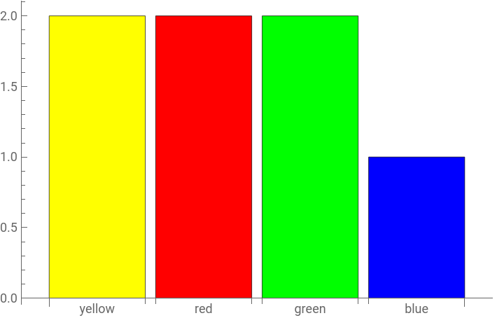
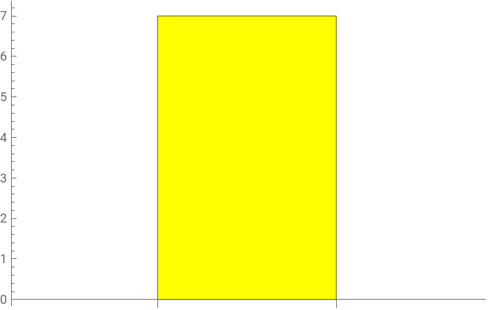
This is how that same BarChart would look, ungrouped
In[]:=
BarChart[{Length[MyFruit]},ChartLabelsAutomatic,ChartStyle{Yellow,Red,Green,Blue}]
Out[]=
- ListLinePlot
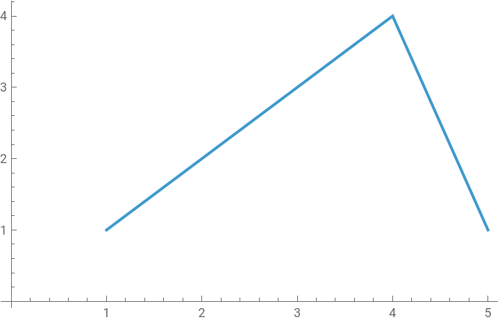
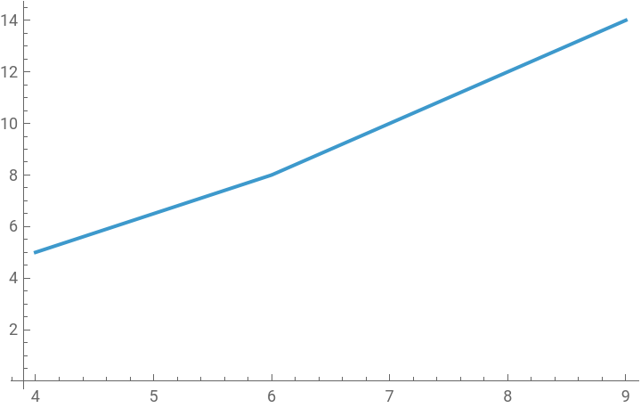
As the name implies, takes in a list of numbers and plots them as a line. Can take in single points, or specific (x,y) pairs.
- ListLinePlot
As the name implies, takes in a list of numbers and plots them as a line. Can take in single points, or specific (x,y) pairs.
In[]:=
ListLinePlot[{1,2,3,4,1}]
Out[]=
In[]:=
ListLinePlot[{{4,5},{6,8},{9,14}}]
Out[]=
When using functions, it's helpful to remember the following:
- Functions only return valid outputs when you give them valid inputs: You can always do a quick look-up of the function to see what the valid inputs are.
- Functions are always written with square brackets, and the input always goes on the inside: Function[ INPUT ] = OUTPUT
- You can sometimes pass through a function as input to another function: Dimensions[Tabular[ ... ]]
- Functions begin with capital letters, and capitalize every new word with no spaces: Dimensions, Tabular, ColumnKeys, BarChart, ListLinePlot, etc
- Functions only return valid outputs when you give them valid inputs: You can always do a quick look-up of the function to see what the valid inputs are.
- Functions are always written with square brackets, and the input always goes on the inside: Function[ INPUT ] = OUTPUT
- You can sometimes pass through a function as input to another function: Dimensions[Tabular[ ... ]]
- Functions begin with capital letters, and capitalize every new word with no spaces: Dimensions, Tabular, ColumnKeys, BarChart, ListLinePlot, etc
How Data is Stored in Wolfram Language
How Data is Stored in Wolfram Language
In the Computational Thinking modules, the standard object used for storing data is a Tabular—this is a technical term for "spreadsheet".
Every column in a Tabular is a variable, like "bill_length" or "race". Every row is a measurement, or association. In statistics, we call these observations or subjects. Associations are written like this in WL:
But in reality, associations don't have to look this scary. If I pass this through the Tabular function, it looks like our typical google sheet or excel file:
And I can continue to add associations (rows) to create a meaningful dataset.
This framework is the backbone of any work involving data in the WL. For more on working with data, please refer to this resource.
Data Visualization
Data Visualization
Much of the data visualization code in the Computation Thinking modules has already been set up for immediate use, but it may be useful to understand how to change certain qualities of a graph without breaking it all (too much).
The basic structure of any plotting function in WL is as follows:
The basic structure of any plotting function in WL is as follows:
In[]:=
PlottingFunction[{
MyData,
OptionName1 -> value1,
OptionName2 -> value2,
OptionName3 -> value3}];
MyData,
OptionName1 -> value1,
OptionName2 -> value2,
OptionName3 -> value3}];
Where MyData, is the data we would like to visualize, and every line after is an quality of the graph we are setting. If I wanted to, for instance, create a histogram using the following tabular, with red bars, a black background, white axes lines, and blue text, I could do so as such:
There are a lot of customization options for each type of graph, so refer to the function's documentation for a comprehensive list and examples on how to use each one. This is the page I used for referencing the options included above for Histogram.
Also notice that if you have a Tabular you must specify which column(s) you would like to visualize. Here, I just wanted to visualize the distribution of ages, so I pulled the first and only column in the data to do so: someData->1.
Also notice that if you have a Tabular you must specify which column(s) you would like to visualize. Here, I just wanted to visualize the distribution of ages, so I pulled the first and only column in the data to do so: someData->1.
Mathematical Background
Mathematical Background
Linear Model
Linear Model
Numerical data points appear quite often in the Computational Thinking modules. When we have this type of data, we are often asking ourselves a question of the form: Can X be used to predict Y? Consider the following dataset from the Biology CT from the AP Research series:
Let's examine penguin bill length and flipper length. We may hypothesize that penguins with bigger bills tend to have longer flippers. Plotting every penguin by bill length and flipper length would produce the following:
Already, it seems that as bill length increases, flipper length also increases. So while one may not necessarily cause the other, it is clear that there is some positive correlation, or relationship between the two variables. How could we quantify this and be certain? One idea, is to draw a simple line that goes straight through the cloud of points above. This is what that would like like:
If that line has a positive slope, then we know that there is indeed a positive relationship between the bill length and flipper length; and if the points are really close to the line, then we know that they have a strong, linear relationship—meaning that we'd expect consistent changes in flipper length (Y) if we were to increase bill length (X) by a certain amount. Ex: If bill length and flipper length have a strong, positive relationship, then we could say that as we increase bill length by 1 mm, we'd be pretty certain that flipper length will increase by some amount. And if we increases bill length again by 1mm, we'd expect flipper length to increase again by the same amount it did before.
Fortunately, there is a function we can use in WL to create this line for us. LinearModelFit is a functions that takes in a predictor (X-value, "bill length" in our scenario) and an outcome (Y-value, "flipper length"), in addition to the dataset they are coming from ("penguins").
Fortunately, there is a function we can use in WL to create this line for us. LinearModelFit is a functions that takes in a predictor (X-value, "bill length" in our scenario) and an outcome (Y-value, "flipper length"), in addition to the dataset they are coming from ("penguins").
There are several pieces of information in this table that all give us a better picture of the linear relationship between our predictor and outcome. Let's begin with the most crucial: the slope coefficient. The value in the first column ('Estimate"), second row ("x"), tell us by how much we would expect our outcome or Y to increase by, on average, for every 1 unit increase in our predictor (X). For our purposes, and by looking at this value alone, we can conclude that: "For every one unit (millimeter) increase in bill length, we would expect, on average, a ≈1.67 units (millimeters). You can also use the Correlation function to determine explicitly how good of a predictor X is of Y:
As the graphic above communicates, we consider any correlation result greater than 0.5 to indicate a strong positive relationship, while a value closer to 0 would be weaker. Having received a value of ≈0.65 above, we know empirically that bill length and flipper length are positively and strongly correlated; furthermore, this answers are original question. Because there is a strong correlation between the two variables, it does in fact seem that bill_length is a good predictor of flipper length.
For more on linear models, follow this link to a more comprehensive video explanation.
For more on linear models, follow this link to a more comprehensive video explanation.
Analysis of Variance (ANOVA)
Analysis of Variance (ANOVA)
Although complex-sounding, ANOVA is simply a tool we use to determine if groups truly differ by some metric. For instance, we may assume that different species of penguins will have different average body masses. On average, we may for instance expect the large, emperor penguin to be heavier, on average, than the smaller gentoo. We would support this notion empirically using ANOVA.
As always, we start with data:
As always, we start with data:
Now, let's pose a question ANOVA can help us solve: Is there a significant difference between the body masses of male and female penguins (observed in the study)? Let us run our ANOVA test using the ANOVA function:
Primarily, an ANOVA test is measuring two thing: within-group variance (how different penguins within the same group are by body mass) and between-group variance (how different penguins from different groups are by body mass). These two values are then divided to get the F-ratio. A high F-ratio indicates that there is a significant difference between the groups (at least by body mass, the measure being compared), whereas a low F-ratio indicates that much of the difference between the groups may be random, and is likely insignificant. F-ratio values around or lower than 1.0 are typically considered low, as the ratio being computed is (between-group)÷(in-group), where a higher between-group value will yield a ratio greater than 1.0. Our results (F-ratio = 72.961) from the table above tell us that, yes, there is a significant difference between male and female penguins in this study (by body mass); moreover, this value indicates that the variance between groups is actually 72 times greater than the variance within-group!
For more on ANOVA, follow this link to a more comprehensive video explanation.
For more on ANOVA, follow this link to a more comprehensive video explanation.
Logistic Regression
Logistic Regression
Logistic regression is very similar to linear regression (linear model), with the small exception that we only use it when the variable we are trying to predict is binary (one thing, or another; heads or tails; short or tall; pass or fail; 0 or 1). To illustrate we will use data from the Social Science CT module from the AP Research series.
As always, we start with data:
As always, we start with data:
Here is a question we can answer using logistic regression: Can we use years of experience an applicant has as an accurate predictor of receiving a call back from an employer? Here, the outcome variable (callback) is binary, since an applicant either receives a call back or not (1 or 0). In WL, we can use the LogitModelFit function to help answer this question:
As with a linear model, we must focus on the first column ("Estimate"), second row ("x") for our main results. This number tells us to what power we raise e (Euler's number), and once we know this, we can express our findings as such: For every one unit increase in X, the odds of getting a Y=1 outcome increases by e^(estimate) times.
Let us frame this concretely. Our estimate is ≈0.039, and so e^(0.039) ≈1.04. This means that for every one unit (year) increase in an applicant's experience, the odds of receiving a call back increases by 1.04 times (or 4%). So, let us suppose that an applicant's chance of getting a callback is 50%. Our model is essentially communicating that with one more year of experience, that same applicant's chance of receiving a call back becomes around 50.97%. This clearly demonstrates that years of experience may only be a weak predictor of callback success, since it leaves an applicant's odds nearly unchanged given more years of said experience.
Let us change the question slightly and run the model again with our new variable: Can we use the race of an applicant as an accurate predictor of receiving a call back from an employer?
Let us frame this concretely. Our estimate is ≈0.039, and so e^(0.039) ≈1.04. This means that for every one unit (year) increase in an applicant's experience, the odds of receiving a call back increases by 1.04 times (or 4%). So, let us suppose that an applicant's chance of getting a callback is 50%. Our model is essentially communicating that with one more year of experience, that same applicant's chance of receiving a call back becomes around 50.97%. This clearly demonstrates that years of experience may only be a weak predictor of callback success, since it leaves an applicant's odds nearly unchanged given more years of said experience.
Let us change the question slightly and run the model again with our new variable: Can we use the race of an applicant as an accurate predictor of receiving a call back from an employer?
Our estimate is ≈0.438, and so e^(0.438) ≈1.5. This means that being white increases an applicant's odds of receiving a call back by 1.5 times (or 50%). So, let us suppose that a black applicant's chance of getting a callback is 50%. Our model is essentially communicating that if that applicant were white, their chance of receiving a call back becomes around 60.78%. This is a significant difference, indicating that race is a stronger predictor of callback success than years of experience.
For more on logistic regression, follow this link to a more comprehensive video explanation.
For more on logistic regression, follow this link to a more comprehensive video explanation.
Moving Average
Moving Average
The moving average, as referenced in the Arts CT of the AP Research series, is what we use when we have a set of values that are considered noisy—or jump between high and low values frequently—and that we would like to get a smoother trend for. Below is an example of the phenomena:
The plot above represents the averages GPAs of students, which fluctuate wildly. Now, let us smooth-out this data using the MovingAverage function:
Below is a comparison of the two graphs, with the raw data in blue, and the moving average in red. The yellow window represents a portion of the data which has been significantly smoothed-out to make the trend here clearer. In fact, we calculate moving averages by taking "windows" of the data, and finding the average for each—instead of just adding all the numbers together and finding the simple average.
For more on the moving average, the Wikipedia article covering it offers an in-depth look at the measure.
Common Errors
Common Errors
Every modern programming language is built on a system of rules that govern how code should be written. Unlike with natural language, small differences in lettering or spacing can make a significant difference in what gets communicated to the computer. Encountering these issues will often make it seem like everything is broken and there's no easy solution to fixing it. In reality, this is far from the truth. Solutions to these issues can be quick, painless, and intuitive with a keen eye and patience. Below are a few common errors and their solutions:
Loading in Necessary Data
Loading in Necessary Data
In this scenario, I am trying to work with some data. Specifically, I would like to view its dimensions:
Why is my output empty? Well, has penguinData been declared yet? In other words, have we told the computer what our data is? Have we loaded it in? The code below first imports the necessary data, then runs the same line as above:
Spelling, Capitalization, and Spacing
Spelling, Capitalization, and Spacing
When writing functions, it is easy to make this simple mistake:
Why is my output just the function I wrote and its input? Well, was the function capitalized? Remember that all functions in Wolfram Language are capitalized, and camel-cased (meaning every new word in the phrase is capitalized and unspaced LikeThis). However, not all things in the WL are written like this; take the resource data from the Arts CT:
The text in red tells us that we have encountered an error. The program is trying to pull the text for Through the Looking Glass from the Wolfram Data Repository, but there is no resource by the name "ThroughTheLookingGlass". Instead, it must be spaced and capitalized as so:
Errors can also be due to simple spelling mistakes. It's best to keep a keen eye for detail while programming in any language, as these are the hardest to spot. Below is code for a data visualization:
So, where is my visualization? The issue is in the function call, where instead of writing "ListLinePlot", we write "ListLinPlot". Here is the corrected code:
Missing/Misplaced Symbols
Missing/Misplaced Symbols
Symbols like semi-colons ; quotation marks "" and brackets [] play an integral role in keeping your code running smoothly and error-free. Here are a few common uses and errors as they relate to symbols in WL.
Semi-colons are used to punctate a line of code, or stop it from printing an output. The following two lines are exactly the same, but only the first one prints, while the second one has a semi-colon at the end, suppressing the output entirely (although, the code still runs for both).
Semi-colons are used to punctate a line of code, or stop it from printing an output. The following two lines are exactly the same, but only the first one prints, while the second one has a semi-colon at the end, suppressing the output entirely (although, the code still runs for both).
Quotes are often used to refer to the name of something, rather than variables themselves. This relationship is illustrated in the code below:
Brackets are everywhere in the WL, mainly because they are essential to writing functions. Code will often break because of a single missing bracket, as such:
The function above is taken from the Arts CT, and calculates a loudness score given some text, but when the cell is ran, it illuminates red: this indicates that there is an error. It may not be clear, but as every opening bracket must have a closing one, we must identify that while we create an opening bracket for Module (second line), we do not write a closing bracket for it at the very end. Here is the fixed version:
Domain-Specific Resources
Domain-Specific Resources
The Computational Thinking modules offer glimpses into the expansive world of Wolfram Language, and provide opportunities to start using these technologies in structured, focused environments. However, if you would like to explore more of what the Wolfram Language has to offer, then you can refer to the following list of web resources:
Mathematics
Mathematics
- Algebraic Computation
- Geometry (Solid)
- Calculus
- Differential Equations
- Number Theory
- Linear Algebra
- Geometry (Solid)
- Calculus
- Differential Equations
- Number Theory
- Linear Algebra
Data Science
Data Science
Natural Sciences
Natural Sciences
Social Sciences
Social Sciences
Arts
Arts