SIR Model with Log-normal infected periods
SIR Model with Log-normal infected periods
Diego Zviovich
Parameters
Parameters
Assume log-normal distribution μ 5.9 days, σ 1.35.
In[]:=
μ=5.9;σ=1.35;maxTime=36000;nbrDivisions=33;population=1000;maxView=180;
Standard model
Standard model
The standard model is deterministic. The infection period is a constant and does not vary from person to person.
In[]:=
sirSoln=ParametricNDSolve[{sd'[t]-βsd[t]id[t]/population,id'[t]==βsd[t]id[t]/population-id[t]/μ,rd'[t]==id[t]/μ,id[0]nbrDivisions,rd[0]0.,sd[0]population-nbrDivisions},{sd,id,rd},{t,0,maxTime},β];
In[]:=
Manipulate[Plot[Evaluate[({sd[β][t],id[β][t],rd[β][t]}/population)/.sirSoln],{t,0,maxView},PlotRangeFull,PlotTheme"Detailed",PlotLegends{"Susceptibles","Infected","Recovered"},FillingAxis,PlotLabel"Fraction of Population by Compartment",FrameLabel{"Time","Population Fraction"}],{{β,1/4.},0,2}]
SIR model assuming a log-normal distribution of infectious period
SIR model assuming a log-normal distribution of infectious period
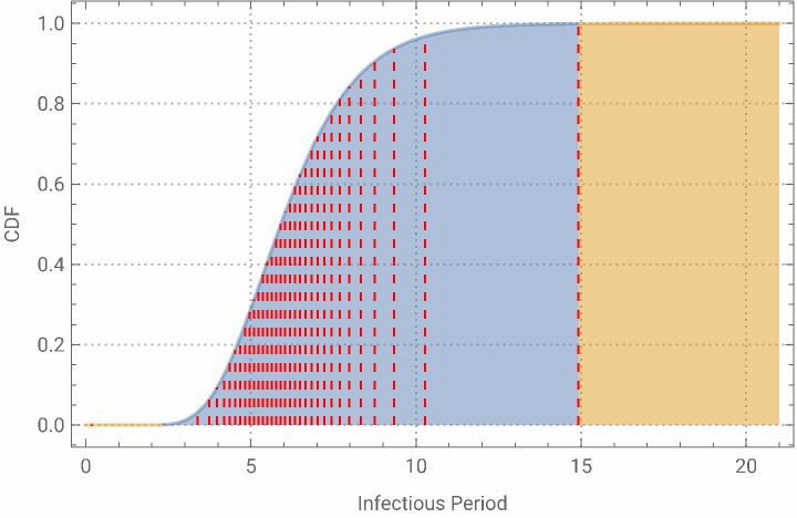
We’ll proceed to divide the infected population in nbrDivisions compartments, each with a different infectious period, determined by the lognormal distribution.
In[]:=
rules=Association[Join[Quiet@Table[ip[n]->x/.First[Solve[CDF[LogNormalDistribution[Log[μ],Log[σ]],x]Rescale[n,{1,nbrDivisions},{0.001,0.999}],x,Reals]],{n,nbrDivisions}],{β1/μ}]];
Our compartments are divided in bins of equal probability of occurrence, each with its specific infectious period.
In[]:=
PlotCDF[LogNormalDistribution[Log[μ],Log[σ]],x],{x,0,21},
Out[]=
In[]:=
Column[{"Infectious Period",TableForm[{PercentForm/@{0.001,0.999},Round[{rules[ip[1]],rules[ip[nbrDivisions]]},0.1]},TableHeadings{{"Quantile","Days"},None}]},AlignmentCenter,FrameAll]
Out[]=
Infectious Period | ||||||
|
Setup of equations and initial conditions.
In[]:=
eqns=Join{s'[t]-βs[t]Sum[i[n][t]/population,{n,nbrDivisions}]},Tablei[n]'[t]βi[n][t]s[t]population-,{n,nbrDivisions},r'[t]Sum,{n,nbrDivisions};
i[n][t]
ip[n]
i[n][t]
ip[n]
In[]:=
initialConditions=Join[Table[i[n][0]1.,{n,nbrDivisions}],{s[0]population-nbrDivisions,r[0]0.}];
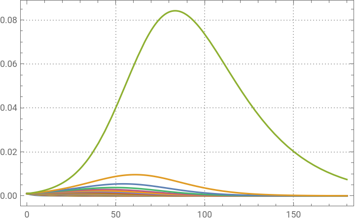
Testing the system with β = 1/μ
In[]:=
soln=Quiet@NDSolve[Join[eqns/.rules,initialConditions],Join[{s,r},Table[i[n],{n,nbrDivisions}]],{t,0,maxTime}];
In[]:=
Plot[Evaluate[Table[i[n][t]/population,{n,nbrDivisions}]/.soln],{t,0,maxView},PlotRangeFull,PlotTheme"Detailed",PlotLegendsNone]
Out[]=
In[]:=
iTotal[t_]:=(Sum[i[n][t],{n,nbrDivisions}]/.soln/.rules)/population
In[]:=
Plot[Evaluate[{s[t]/population,iTotal[t],r[t]/population}/.soln/.rules],{t,0,maxView},PlotRangeFull,PlotTheme"Detailed",PlotLegends{"Susceptibles","Infected","Recovered"},FillingAxis,PlotLabel"Fraction of Population by Compartment",FrameLabel{"Time","Population Fraction"}]
Out[]=


Parametrizing the model
Parametrizing the model
Set up the solution based on the contact rate value β as a parameter
In[]:=
solnParametric=ParametricNDSolve[Join[eqns/.KeyDrop[rules,β],initialConditions],Join[{s,r},Table[i[n],{n,nbrDivisions}]],{t,0,maxTime},β];
In[]:=
iTotalParametric[β_,t_]:=ParallelSum[i[n][β][t],{n,nbrDivisions}]/.solnParametric
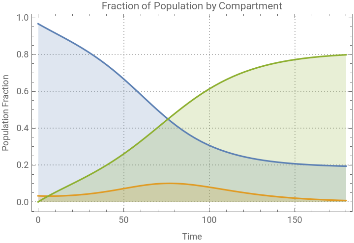
The chart indicates, as expected, that the deterministic model is more conservative. Peak will be higher and happen faster when taking into consideration the probability distribution of the infectious period.
Comparing the difference in results between the fixed infectious period value model and the log-normal model
Comparing the difference in results between the fixed infectious period value model and the log-normal model
We can visualize that when we set up the infectious period as a stochastic variable, the epidemic will run its course at a lower value of β.
In[]:=
Manipulate[Quiet@Plot[Evaluate[{id[β][t]/.sirSoln,iTotalParametric[β,t]}/population],{t,0,maxView},PlotRangeFull,PlotTheme"Detailed",PlotLegends{"Deterministic","LogNormal"},FillingAxis],{{β,0.135},0,2},SynchronousInitializationFalse,SynchronousUpdatingFalse]
When tracking the number of remaining susceptible, it can be observed how much conservative using the deterministic model is. While low values of β would reflect almost no contagion spread across of the population in the deterministic model, the effect of the lognormal distribution of the infectious period takes its toll in the susceptible population.
In[]:=
Manipulate[Quiet@Plot[Evaluate[{sd[β][t]/.sirSoln,s[β][t]/.solnParametric}/population],{t,0,tMax},PlotRange{Automatic,{0,1}},PlotTheme"Detailed",PlotLegends{"Deterministic","LogNormal"},FillingAxis],{{β,0.135},0,0.4},{{tMax,maxView},maxView/3,maxTime},SynchronousInitializationFalse,SynchronousUpdatingFalse]
Effect of the infectious period distribution on the SIR model
Effect of the infectious period distribution on the SIR model
We have observed in the charts above that indeed the epidemic takes off at lowest values of contact rates when we take the infectious period log normal distribution into consideration.
Given the current values of μ and σ, let’s proceed to calculate the where the epidemic starts taking hold.
To do so, we’ll calculate the second derivate of the recovered population at maxTime with respect to the value of β.
Given the current values of μ and σ, let’s proceed to calculate the where the epidemic starts taking hold.
To do so, we’ll calculate the second derivate of the recovered population at maxTime with respect to the value of β.
In[]:=
βDeterministic=β/.First@Last@FindMaximum[rd''[β][maxTime]/.sirSoln,{β,0,2},AccuracyGoal20,PrecisionGoal18,WorkingPrecision40];ptβDeterministic=Point[{βDeterministic,(sd[βDeterministic][maxTime]/population)/.sirSoln}];βStochastic=β/.First@Last@FindMaximum[r''[β][maxTime]/.solnParametric,{β,0,2},AccuracyGoal20,PrecisionGoal18,WorkingPrecision40];ptβStochastic=Point[{βStochastic,(s[βStochastic][maxTime]/population)/.solnParametric}];
In[]:=
Plot[Evaluate[{sd[β][maxTime]/.sirSoln,s[β][maxTime]/.solnParametric}/population],{β,0,1},PlotRangeFull,PlotLegends{"Deterministic","LogNormal"},Epilog{Red,PointSize@Medium,ptβDeterministic,ptβStochastic}]
Out[]=
For this set of parameters, the β for the stochastic process is a significant fraction lower than the determinstic one.
In[]:=
Column[{"β (Contact Rates)",TableForm[Round[{βStochastic,βDeterministic,βStochastic/βDeterministic},0.001],TableHeadings{{"Stochastic","Deterministic","Ratio"},None}]},FrameAll]
Out[]=
β (Contact Rates) | ||||||
|
An analytic approach to the problem
An analytic approach to the problem
where β is the contact rate, s[t] is the number of susceptibles, N is the total population and μ is the infectious period. Assuming that i[t] 0 then s[t] /N 1, we obtain
If the contact rate is Log-Normally distributed then