For many applications in simulation, dynamical systems, robotics, machine learning, etc., we need random vectors that are uniformly distributed in multidimensional spheres. The number of dimensions can be very large, ruling out rejection methods (generate randoms in a d-cube, then filter out points not in the sphere). We exhibit two efficient methods, one geometric and one statistical. The statistical method is proved by invoking an ancient and beautiful theorem attributed to Archimedes.
Abstract
Abstract
Can we generate spherically symmetric uniform randoms starting with rectangularly symmetric, uniform randoms? Yes, but it takes care to do it efficiently. Rejection methods — generating rectangularly symmetric, uniform randoms and then throwing out those that are not in the -ball — are crippled: only one in a trillion endpoints in the 27-cube is also in the 27-ball; the ratio gets worse exponentially as increases. We need spherically symmetric uniform randoms in the thousands of dimensions for robots or even in the billions of dimensions for neural networks.
d
d
We exhibit two computational methods — one geometrical, the other statistical — that scale efficiently with for generating pseudorandom vectors uniformly and symmetrically on the surface and in the interior of the unit hypersphere of dimension .
d
d
Though no method here is novel, descriptions available to me are unsatisfactory. The contributions of this note are proofs, executable specifications of algorithms, and numerical demonstrations.
Definitions
Definitions
The unit -ball is the interior of a hypersphere, hyper meaning of any dimension. The unit -ball is the set of all real -vectors rooted at the origin, , such that ++⋯+<1. The unit -sphere is the boundary of the -ball, that is, the set of all real -vectors such that ++⋯+=1.
d
d
d
(,,…,)∈
x
1
x
2
x
d
d
2
x
1
2
x
2
2
x
d
d
d
d
2
x
1
2
x
2
2
x
d
The unit -cube is the set of all real -vectors such that each coordinate is absolutely bounded by unity, inclusively, that is, where . The unit -ball, -sphere, and -cube are also said to have radius 1, diameter 2.
d
d
-1≤≤1
x
i∈[1..d]
d
d
d
We do not distinguish between the mathematical procedure of sampling a distribution and the computational procedure of generating pseudorandoms according to a distribution. Likewise, we do not distinguish between mathematical true randoms and computational pseudorandoms.
Generating randoms uniformly means the same as generating uniform randoms. Generating randoms symmetrically means the same as generating symmetric randoms. Symmetrically means independently of geometrical direction.
Uniform Randoms in the d-Cube
Uniform Randoms in the -Cube
d
Given an efficient method for generating uniform random scalars in the real interval — in the 1-cube — it is easy and efficient to generate rectangularly symmetric, uniform randoms in the -cube: generate randoms for each of the coordinate components independently.
[-1..1]
d
d
Can we generate spherically symmetric uniform randoms starting with rectangularly symmetric, uniform randoms? Yes, but it takes care to do it efficiently. Rejection methods — generating rectangularly symmetric, uniform randoms and then throwing out those that are not in the -ball — are crippled: only one in a trillion endpoints in the 27-cube is also in the 27-ball; the ratio gets worse exponentially as increases.
d
d
Consider points (vector endpoints) uniformly distributed in the unit 2-cube, i.e., the unit square. The resulting pairs are not uniform with angle, therefore not spherically symmetric. The following diagrams illustrate: here are points uniformly distributed in the 2-cube:
(x,y)
Out[]=
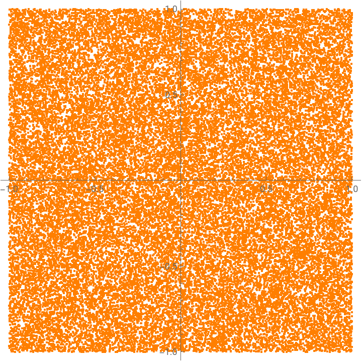
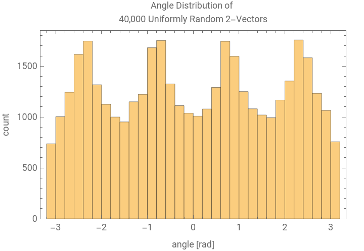
There are too many points in the corners, at , and their negatives:
ArcTan[1,1]=0.7854
ArcTan[-1,1]=2.3562
Out[]=
Rejection Method: Impractical
Rejection Method: Impractical
We could reject, i.e., remove points in the unit -cube that are not in the unit -ball. Those would be points with radial component — Euclidean norm — greater than 1. However, rejection does not scale. As grows, the number of corners goes up as and almost all points are in the corners, outside the -ball. To see this this, consider the ratio of the volume of a unit -ball to the volume of a unit -cube.
d
d
d
d
2
d
d
d
What is the volume of a unit -cube? Answer: . What is the volume of a unit -ball? (see https://en.wikipedia.org/wiki/Volume_of_an_n-ball)
d
d
2
d
Answer for integer :
d
In[]:=
ClearAll[vBall];vBall[d_,r_:1]:=
;Table<|"dimension"d,"ball volume"vBall[d],"cube volume","cube/ball ratio"NvBall[d]|>,{d,1,10}//MatrixForm
|
d
2
d
2
Out[]//MatrixForm=
dimension1,ball volume2,cube volume2,cube/ball ratio1. |
dimension2,ball volumeπ,cube volume4,cube/ball ratio1.27324 |
dimension3,ball volume 4π 3 |
dimension4,ball volume 2 π 2 |
dimension5,ball volume 8 2 π 15 |
dimension6,ball volume 3 π 6 |
dimension7,ball volume 16 3 π 105 |
dimension8,ball volume 4 π 24 |
dimension9,ball volume 32 4 π 945 |
dimension10,ball volume 5 π 120 |
for arbitrary real dimensions, the plot must be logarithmic to be useful. Notice the volume ratio is about for .
-12
10
d=27
In[]:=
ClearAll[vBall];vBall[d_,r_:1]:=;
d/2
π
d
r
Gamma[1+d/2]
Out[]=
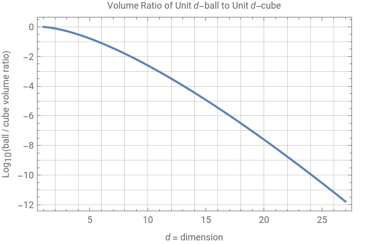
The ratio of ball-to-cube volume in 27 dimensions is one trillionth, so the rejection method generates a trillion times more points than it keeps. The computer does 1 trillion times more work than it ought to do. Rejection is impractical for even moderately large .
d
Radial Symmetry
Radial Symmetry
Observe that a multivariate Gaussian or multinormal distribution is radially symmetric. Sampling from , and similarly, then noticing that and are independent (the probability of their occurring simultaneously is the product of their individual probabilities), we get ×=. A similar construction extends to any number of dimensions.
x
-
2
x
2
2π
y
x
y
-
2
x
2
2π
-
2
y
2
2π
-+
1
2
2
x
2
y
2π
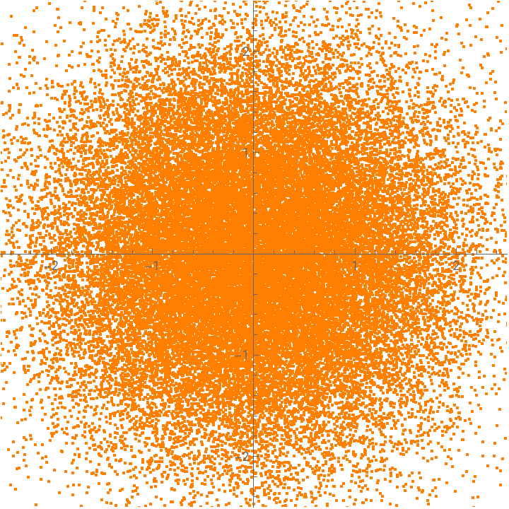
The multinormal distribution is radially symmetric because it depends only on the radius squared, +, not on the azimuth angle. But it is not radially uniform, as the following figure demonstrates:
2
x
2
y
In[]:=
show2D$[RandomVariate[
MultinormalDistribution[IdentityMatrix[2]]
,40000],2.5]Out[]=
Radial Uniformity
Radial Uniformity
From Symmetry to Uniformity
From Symmetry to Uniformity
Efficient Geometrical Construction
Efficient Geometrical Construction
sampleDBall
sampleDBall
The following plots illustrate points uniformly distributed in radius in two and three dimensions, and thus uniformly distributed in the 2-ball and in the 3-ball, respectively:
Uniformity Statistics
Uniformity Statistics
It’s well and good to appear to be uniform, but we must demonstrate uniformity with statistics.
Shell Statistics
Shell Statistics
A rigorous Chi-squared test would give the probability that each shell is not drawn from the same uniform distribution. The “eyeball” agreement between empirical and expected standard deviations is good enough that a rigorous Chi-squared test does not seem worth the effort.
Sampled Shell Counts
Sampled Shell Counts
Two Dimensions
Two Dimensions
Three Dimensions
Three Dimensions
Six Dimensions
Six Dimensions
Sixteen Dimensions
Sixteen Dimensions
276 Dimensions
276 Dimensions
Cubie Statistics
Cubie Statistics
Two Dimensions
Two Dimensions
There are already, even in two dimensions, a noticeable number of deficiently populated cubies (the tail to the left of the peak above). These are the cubies crossing the circle and in the corners outside the circle.
Three Dimensions
Three Dimensions
In three dimensions, the number of deficient cubies is larger than “noticeable.”
Six Dimensions
Six Dimensions
In six dimensions, the deficient cubies dominate the statistics.
Twenty-Seven Dimensions
Twenty-Seven Dimensions
In twenty-seven dimensions, virtually all the cubies are deficient.
Efficient Statistical Construction
Efficient Statistical Construction
Why does this work? Why reject two coordinates at random, instead of one or three or seventeen?
Theorem 1
Theorem 1
Proof
Proof
We prove the theorem first for three dimensions, then argue by extension to dimensions greater than three.
As before, generate spherically uniform 3-vectors of unit length — on the 3-sphere — by sampling the 3-dimensional multinormal distribution, then normalizing the vectors:
What is the 2D distribution at this step?
Lemma 1
Lemma 1
The following illustrates five belts in 3D:
Proof of the Hatbox Theorem
QED Hatbox Theorem ■
We claim that each annulus contains the same number of points, statistically.
The following illustrates that all annuli have, statistically, the same numbers of points.
QED Lemma 1 ■
Therefore each band has the same density.
Two Dimensions
Two Dimensions
276 Dimensions
276 Dimensions
QED Theorem 1 ■
CITE THIS NOTEBOOK
CITE THIS NOTEBOOK
Archimedes' Hatbox — Hyperspherical Pseudorandom Vectors
by Brian Beckman
Wolfram Community, STAFF PICKS, December 11, 2023
https://community.wolfram.com/groups/-/m/t/3081911
by Brian Beckman
Wolfram Community, STAFF PICKS, December 11, 2023
https://community.wolfram.com/groups/-/m/t/3081911