ABSTRACT (original article): We describe a simple method for tracking solutions of nonlinear equations f(u,α) = 0 through turning points (also known as limit or saddle-node bifurcation points). Our implementation makes use of symbolic software such as Mathematica to derive an exact system of nonlinear ODE equations to follow the solution path, using a parameterization closely related to arc length. We illustrate our method with examples taken from the engineering literature, including examples that involve nonlinear boundary value problems that have been discretized by finite difference methods. Since the code requirement to implement the method is modest, we believe the method is ideal for demonstrating continuation methods in the classroom. CITATION (original article): Higgins, B. G., & Binous, H. (2010). A Simple Method for Tracking Turning Points in Parameter Space. JOURNAL OF CHEMICAL ENGINEERING OF JAPAN, 43(12), 1035–1042. DOI: https://doi.org/10.1252/jcej.10we122
We use the Homotopy method described in detail in Ref. 1 in order to determine the local and global extrema. To illustrate our procedure, let us consider the following constrained optimization problem:
MinorMaxf(x,y)=xcos(y)+0.1-ysin(x)
2
x
s.b.t.
g(x,y)=+5-3y=0
2
x
xandy≤10
Contours of
f(x,y)=xcos(y)+0.1-ysin(x)
2
x
In[]:=
p1=ContourPlot[xCos[y]+0.1x^2-ySin[x],{x,-10,10},{y,-10,10},Contours20,FrameLabel{Style["x",14,Italic],Style["y",14,Italic]}]
Out[]=
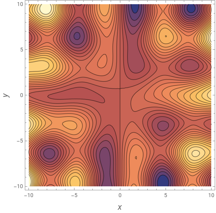
Plot of
g(x,y)=+5-3y=0
2
x
In[]:=
p2=ContourPlot[x^2-3y+5,{x,-10,10},{y,-10,10},Contours{0},ContourShadingNone,ContourStyle{Thick,Darker@Green}]
Out[]=
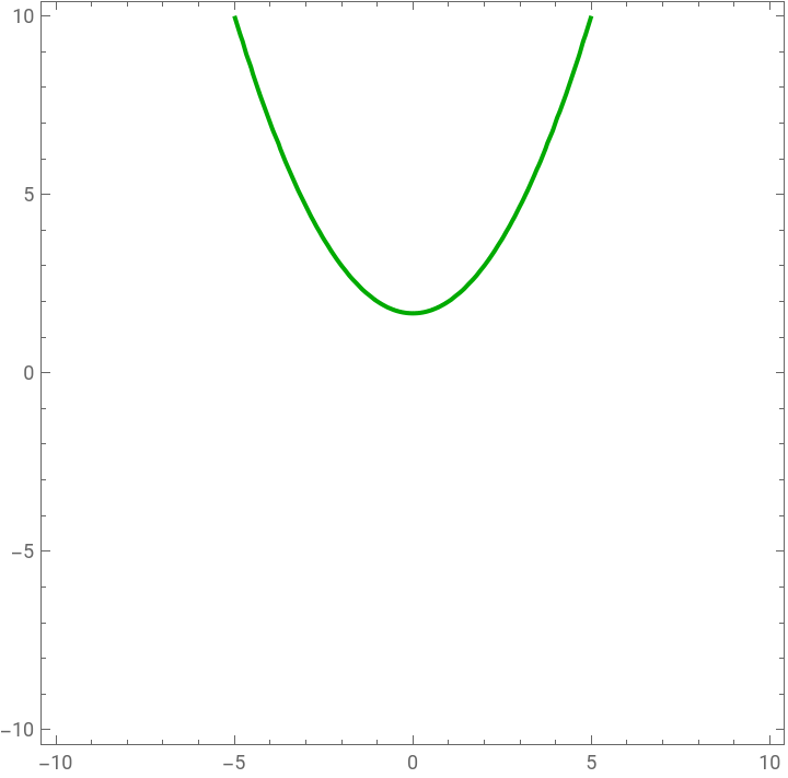
Using FindMinimum and FindMaximum to fetch potential extrema (both local and global)
In[]:=
{min,LocMinpoint}=FindMinimum[{xCos[y]+0.1x^2-ySin[x],x^2-3y+50,-10≤x≤10,-10≤y≤10},{x,3},{y,-9}]
Out[]=
{-4.36959,{x2.12728,y3.17511}}
In[]:=
{min,LocMinpoint2}=FindMinimum[{xCos[y]+0.1x^2-ySin[x],x^2-3y+50,-10≤x≤10,-10≤y≤10},{x,3},{y,9}]
Out[]=
{6.81278,{x4.77033,y9.252}}
In[]:=
{max,Maxpoint}=FindMaximum[{xCos[y]+0.1x^2-ySin[x],x^2-3y+50,-10≤x≤10,-10≤y≤10},{x,4},{y,9}]
Out[]=
{9.93669,{x4.04131,y7.11073}}
In[]:=
{min,LocMaxpoint}=FindMaximum[{xCos[y]+0.1x^2-ySin[x],x^2-3y+50,-10≤x≤10,-10≤y≤10},{x,-2.2},{y,3.3}]
Out[]=
{5.31803,{x-2.22637,y3.31891}}
In[]:=
{min,LocMaxpoint2}=FindMaximum[{xCos[y]+0.1x^2-ySin[x],x^2-3y+50,-10≤x≤10,-10≤y≤10},{x,-4.2},{y,9.3}]
Out[]=
{-2.21359,{x-4.81991,y9.41051}}
In[]:=
{min,Minpoint}=FindMinimum[{xCos[y]+0.1x^2-ySin[x],x^2-3y+50,-10≤x≤10,-10≤y≤10},{x,-4.7},{y,6.3}]
Out[]=
{-6.71698,{x-3.98371,y6.95664}}
Loci of of all extrema when x and y ≤ 10
In[]:=
Show[p1,p2,Graphics[{Darker@Magenta,PointSize[0.025],Point[{x,y}/.Minpoint],Darker@Yellow,Point[{x,y}/.LocMinpoint2],Darker@Red,Point[{x,y}/.LocMinpoint],Darker@Blue,Point[{x,y}/.Maxpoint],Darker@Green,Point[{x,y}/.LocMaxpoint2],Darker@Cyan,Point[{x,y}/.LocMaxpoint]}]]
Out[]=
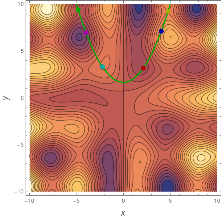
Let us construct the Lagrangian of our optimization problem where l is the Lagrangian multiplier
In[]:=
Lagrangian[x_,y_,l_]:=xCos[y]+0.1x^2-ySin[x]+l(x^2-3y+5)
Loci of of all extrema are the roots of eq1, eq2 and eq3 obtained by setting the partial derivatives of the Lagrangian with respect to x, y and l equal to zero.
In[]:=
eq1=D[Lagrangian[x,y,l],x]0
Out[]=
0.2x+2lx-yCos[x]+Cos[y]0
In[]:=
eq2=D[Lagrangian[x,y,l],y]0
Out[]=
-3l-Sin[x]-xSin[y]0
In[]:=
eq3=D[Lagrangian[x,y,l],l]0
Out[]=
5+-3y0
2
x
At t=0 where solve a simple problem with know solution. Here, we chose a system of three linear equations.
In[]:=
f1=-(t-1)(x+y+l-1)+t(eq1[[1]]);f2=-(t-1)(x+2y+l+1)+t(eq2[[1]]);f3=-(t-1)(x+y-l+1)+t(eq3[[1]]);
In[]:=
NSolve[{x+y+l-10,x+2y+l+10,(x+y-l+1)0},{x,y,l}]
Out[]=
{{x2.,y-2.,l1.}}
The Jacobian matrix is now formed
In[]:=
MyGrad[fon_,var_List]:=D[fon,#]&/@var(*Jacobianmatrix*)
In[]:=
J=Outer[D,{f1,f2,f3},{x,y,l,t}];Dimensions[J]
Out[]=
{3,4}
We are now ready to implement our Homotopy method
s is a continuation parameter
In[]:=
Js=J/.xx[s]/.y->y[s]/.ll[s]/.tt[s];
In[]:=
RHS=FlattenTableDet[Transpose[Drop[Transpose[Js],{i}]]],{i,1,4};
i
(-1)
In[]:=
Eqns=Thread[{x'[s],y'[s],l'[s],t'[s]}RHS];
In[]:=
IC={x[0]2,y[0]-2,l[0]1,t[0]0}
Out[]=
{x[0]2,y[0]-2,l[0]1,t[0]0}
WhenEvent keeps track of the extrema, which are obtained for t=1
In[]:=
{sol,extremapoints1}=Flatten[Reap@Quiet@NDSolve[Flatten@{Eqns,IC,WhenEvent[t[s]1&&Abs[x[s]]≤10&&Abs[y[s]]≤10,{Sow[{s,t[s],x[s],y[s],x[s]^2+5-3y[s],x[s]Cos[y[s]]+0.1x[s]^2-y[s]Sin[x[s]]}]}]},{x,y,l,t},{s,-10,10},AccuracyGoal10],1]
Out[]=
xInterpolatingFunction
,yInterpolatingFunction
,lInterpolatingFunction
,tInterpolatingFunction
,{{-0.248809,1.,2.12728,3.17511,-4.93185×,-4.36959},{-0.253764,1.,4.04131,7.11073,-4.86956×,9.93669},{-0.254769,1.,4.77033,9.252,-5.72514×,6.81278}}


-7
10
-7
10
-8
10
We repeat this time with (t-1) factor instead of (1-t) factor
The Jacobian matrix is now formed
We are now ready to implement our Homotopy method
s is a continuation parameter
WhenEvent keeps track of the extrema obtained for t=1
Final checks indicate that Homotopy is capable of finding all extrema without the need of trying various good initial guesses.
In addition, we did not need to know a priori the exact number of these extrema!!!
In addition, we did not need to know a priori the exact number of these extrema!!!
Loci of of all extrema obtained with Homotopy
Loci of of all extrema when we solve the system {eq1=0, eq2=0, eq3=0} for several values of the initial guesses
Loci of of all extrema when we use FindMinimum and FindMaximum for a selection of values of the initial guesses
Final check and solution by substitution
CITE THIS NOTEBOOK
CITE THIS NOTEBOOK
All global and local extrema of a function by homotopy
by Housam Binous and Ahmed Bellagi
Wolfram Community, STAFF PICKS, July 3, 2025
https://community.wolfram.com/groups/-/m/t/3490902
by Housam Binous and Ahmed Bellagi
Wolfram Community, STAFF PICKS, July 3, 2025
https://community.wolfram.com/groups/-/m/t/3490902