Can a single reassuring measurement point be enough to trust a quantum simulation?
The recorded eight-qubit result looks reassuring only against one target. At t=0.5 the measured staggered magnetization is 0.59662, 1.20 sampling SE from the matching four-step ideal circuit's 0.60245. The new exact-model value is 0.60748, 2.23 SE away and outside the nominal pointwise 95% sampling interval. We selected this example after inspecting the data: it is the only magnetization interval among 13 positive-time rows to include its matching discretized circuit reference. This is a target-dependent, post-hoc comparison, not a generally accurate curve. Meanwhile, its measured energy is −0.38055 per spin, versus −0.86178 for that circuit. A single summary has missed a serious discrepancy.
The central result is a mismatch between two measurements of the same intended dynamics. We start with that result, examine the original timing comparison, and then build the quantum-mechanics tools needed to understand both.
We will follow that discrepancy from the Hamiltonian to the measured bitstrings, and then to a 60-qubit stress case. The aim is to learn how to inspect a quantum result: combine observables, understand the approximation, and ask a separate question about noise.
All IBM results here were recorded on 12 October 2026. This article reuses those files. Rebuilding the post needs no IBM account, token, network connection or QPU allocation. Historical simulations and six-qubit teaching outputs are retained. A local eight-qubit reference, computed once and saved, compares exact evolution with Strang k=1,2,4,8 at t=0.5; it uses WolframScript and no QPU. Its numerical outputs are bundled, so reading or rebuilding this article does not repeat that calculation.
Start here: reproduce the saved analysis
Start here: reproduce the saved analysis
Keep this notebook, QuantumDynamicsArticle.wl, QuantumDynamicsData.wxf, GHZPhaseCoherence.wl, GHZValidation.wxf and quantum-diagnostics-hero.png in one folder. Use Wolfram Language 15.0.1 and Quantum Framework 2.1.1, the recorded environment, or record and check your own versions. If the paclet is missing, install the released Wolfram/QuantumFramework once before loading the companion. No Python runtime or IBM credentials are needed for the saved-count analysis. The evaluated outputs are already included; reading them needs no reevaluation.
In[]:=
Get[FileNameJoin[{NotebookDirectory[],"QuantumDynamicsArticle.wl"}]];allowNewQPU=False;QDInitialize[NotebookDirectory[]]
Out[2]=
StatusPASS,ModeSaved-data replay,DataLoadedTrue,QPUCalls0,WolframVersion15.0.1 for Mac OS X ARM (64-bit) (July 2, 2026)
In[]:=
QDAudit[]
The audit recomputes 15 observable rows from 32 saved measurement circuits and checks 131,072 outcomes. It is classical arithmetic on recorded counts. Package installation and IBM access are separate, optional actions.
The opening load also loads GHZPhaseCoherence.wl and its saved GHZValidation.wxf. Keep both WL sources and both WXF files beside this notebook. All GHZ plots, controls and frames have their complete generators in that supplied source. No GHZ validation is triggered by loading or replay.
What this experiment adds
What this experiment adds
The original contribution is this recorded mixed-field-Ising experiment and its reproducible audit—not a new Hamiltonian, product formula or access API. The key evidence combines two measurement bases, two full-string echoes and classical-reference checks across 8–60 qubits.
The complete selection screen is open below: all 13 positive-time magnetization gaps, expressed in their own sampling standard errors. Only one row is inside its pointwise ±1.96 interval. This is a selected counterexample, not a typically accurate hardware curve.
In[]:=
QDSelectionScreen[]
Out[4]=
In[]:=
QDFigure["13-key-results"]
Out[5]=

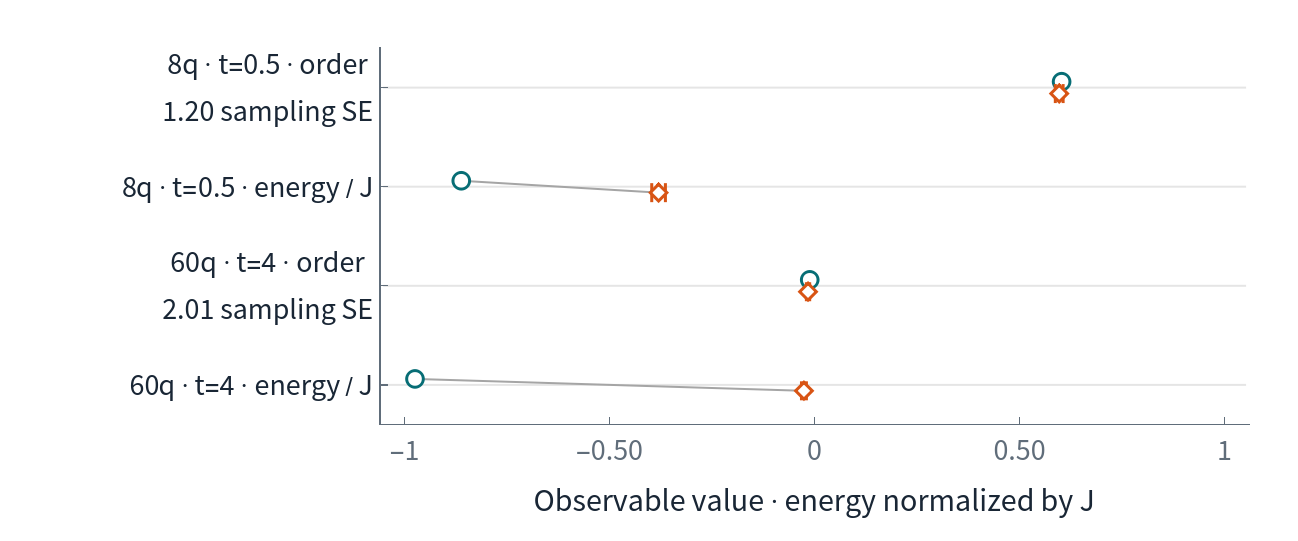
At eight qubits, a selected magnetization point is only 1.20 sampling SE from its ideal circuit value while energy differs by 0.481 per spin. At sixty qubits, small absolute magnetization accompanies a 0.949 energy gap. The eight-qubit example was selected after inspecting all 13 positive-time rows; the sixty-qubit order difference is 2.01 SE and narrowly misses its pointwise interval. These are complementary warnings, not two claims of statistical agreement.
The starting point: why 60 qubits caught our attention
The starting point: why 60 qubits caught our attention
The original notebook began with a striking comparison of classical scaling and an actual 60-qubit IBM run. This graphic is central to the story. Here we reconstruct it in Wolfram Language from the original saved timing data, with the complete generating function supplied.
In[]:=
QDFigure["original-scaling"]
Out[6]=
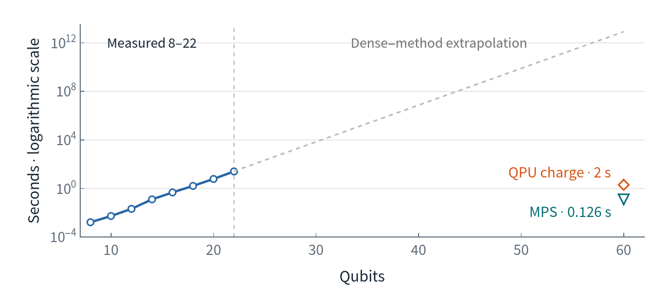
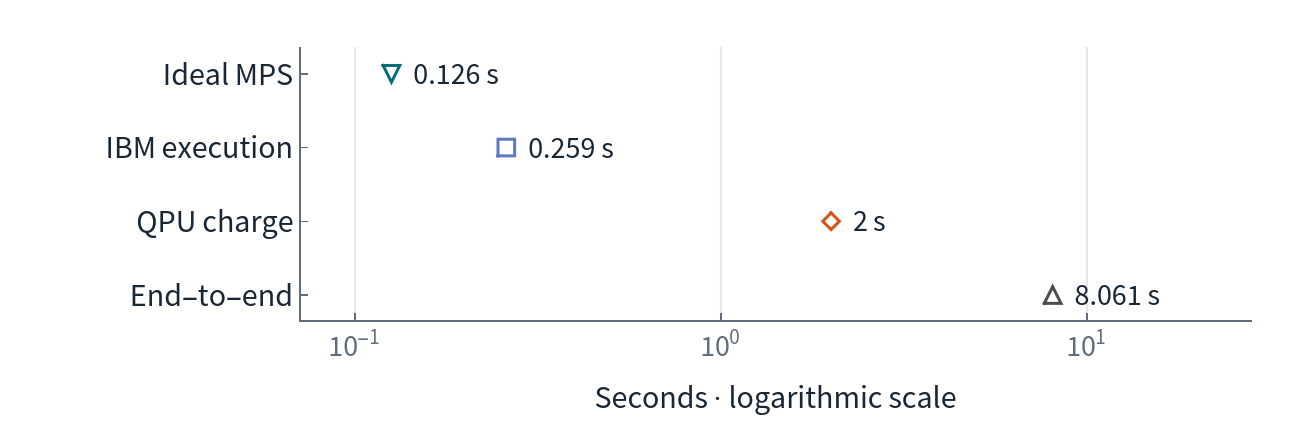
Wolfram reconstruction of the original archived comparison; no timings were remeasured. Blue points are measured Wolfram dense-array timings; the dashed gray line extrapolates that method alone. The orange diamond is the measured IBM charge time. The teal downward triangle is historical Qiskit Aer ideal MPS sampling of the shallow hardware circuit. The dense baseline applies one Hadamard layer: its ideal output is a product state, representable with bond dimension one. It is not a speedup bound.
Read the dense-scaling panel as a lesson about representation and structure. A full state vector becomes exponentially expensive to store and update. Here the steep baseline measures the cost of materializing and updating that representation, even for a simple Hadamard-only product-state circuit. It was measured from 8 to 22 qubits at depth 1; the dashed extension is a descriptive fit to that implementation. But the ideal MPS point at 60 qubits is crucial: the shallow circuit used in the original hardware experiment was still classically tractable. A 60-qubit register does not force every simulation to materialize 2⁶⁰ amplitudes.
The fitted model is T(n) = Exp[a + b n] seconds, with a ≈ −12.04133 and b ≈ 0.696460. We recompute the natural-log least-squares fit, its residuals and log-scale R² (≈0.99831) from the archived timings. A good fit over 8–22 qubits does not validate its extension to 60. The local slope of log time also changes across these measured sizes; the returned log residuals should be inspected rather than treating a high R² as evidence of a universal exponential law. That extension has no calibrated prediction interval; memory limits, implementation changes and different algorithms prevent a literal runtime prediction.
In[]:=
QDDenseFitAudit[]
Out[7]=
StatusPASS,ModelSeconds = Exp[a + b n]; least squares on natural log seconds,a-12.0413,b0.69646,MeasuredQubits{8,10,12,14,16,18,20,22},BenchmarkDepth1,CircuitHadamard-only; ideal product state; bond dimension one,LogResiduals{0.0669031,-0.143332,-0.176286,0.22617,0.151161,-0.0027545,-0.0795574,-0.0423049},LogRSquared0.998307,MaxRelativeArchivedExtrapolationDifference3.19744×,ExtrapolationLimitDescriptive fit to one implementation, 8-22 qubits. No validated error band or prediction for other simulators; memory constraints invalidate literal execution at 60 qubits.
-14
10
The timing panel records four distinct timings for that original shallow 60-qubit experiment, with 1,000 samples:
In[]:=
QDSummaryTable[1]
Out[8]=
The ideal classical samples and the noisy hardware samples do not have the same accuracy meaning. The dense baseline also uses a different circuit. Therefore neither the long-range dense extrapolation nor a ratio of these timings proves quantum advantage. The figure demonstrates why an apparently dramatic comparison must be read alongside an appropriate classical alternative.
This leads to a more scientifically useful next question: can we use a quantum circuit to follow a specified physical model, and test whether its measured answer is reliable? That motivates the mixed-field Ising experiment below. Its expanded workload has 32 circuits, 131,072 outcomes and 37 seconds of charged QPU time. The original graphic's 2 seconds and the later 37 seconds belong to different recorded jobs; they must not be merged into one benchmark.
Before the model: what does a measurement actually tell us?
Before the model: what does a measurement actually tell us?
A qubit has two computational basis states, written |0⟩ and |1⟩. These are quantum states, not the classical numbers zero and one. For n qubits there are 2ⁿ basis states, one for each binary string. A pure state assigns a complex amplitude to every string; normalization makes the squared amplitudes add to one. The Born rule turns those amplitudes into the probabilities of Z-basis outcomes.
ψ⟩= ∑ b∈ n {0,1} c b |
∑ b 2 | c b p Z 2 | c b |
One shot returns one string b. It does not reveal the list of amplitudes or their relative phases. Repeating the experiment estimates probabilities. It therefore matters which measurement basis we choose and which summary of the resulting strings we retain.
An observable is represented by a Hermitian operator. In a chosen basis it is a matrix; its eigenvalues are the possible measurement values. For a spin-½ system, the Pauli Z observable assigns +1 to |0⟩ and −1 to |1⟩. The Pauli X observable distinguishes superpositions along a different axis and exchanges |0⟩ with |1⟩. These ±1 values use the Pauli convention; the physical spin component is ℏZ/2.
Z=
| ||||||||
Z0⟩=0⟩,Z1⟩=−1⟩ |
The density matrix describes both a pure state and a statistical mixture. For a pure state it is the outer product shown below; for a mixture it is a probability-weighted average of such matrices. Its trace is one. The trace rule below gives the average of an observable over repeated preparations; the final equality is the single-qubit Z example. In a chain, Xⱼ or Zⱼ acts on site j and as the identity on every other site.
ρ=ψ⟩⟨ψ,⟨O⟩=Tr(ρO) |
⟨Z⟩= p Z p Z |
Here is the smallest counterexample behind this entire article. A qubit in the pure |+⟩ state and a completely mixed qubit both give 0 and 1 with probability one half when measured in Z. Their X averages are different (I denotes the identity operator):
+⟩= 0⟩+1⟩ 2 ρ mix I 2 |
⟨X⟩ + ⟨X⟩ mix |
In the computational basis the two basis states are column vectors, and the Hadamard is the following 2×2 matrix. Matrix multiplication transforms amplitudes, not probabilities.
Its first output amplitude adds the two input amplitudes; its second subtracts them. For |+⟩ the second amplitude cancels, whereas for |−⟩ the first cancels. This constructive/destructive interference makes the otherwise invisible relative sign observable after the basis change. Both inputs have the same Z probabilities before that change. A Hadamard on a single qubit creates a superposition from |0⟩, but applying Hadamards separately to a product state does not create entanglement. The gate is its own inverse; the Hamiltonian H below is a different object.
The |+⟩ and |−⟩ states are the eigenstates of X, with eigenvalues +1 and −1. Write the Hadamard gate as h, to distinguish it from the Hamiltonian H. It maps the X eigenstates to the computational basis. Thus a Hadamard followed by Z readout has X statistics; the final trace identity below also verifies the |+⟩ average directly.
Matching even the complete Z distribution cannot distinguish those states. Matching only one number, such as magnetization, supplies still less information. The eight- and sixty-qubit results below turn that elementary observation into a practical diagnostic. Energy supplies an additional, physically motivated constraint; even agreement in both energy and magnetization would not by itself reconstruct or certify the full state. For a systematic account of measurements and state reconstruction, see IBM Quantum Learning.
Explore the saved results interactively
Explore the saved results interactively
The static preview below is saved for reading and printing. The following Wolfram notebook control selects among plots prepared from the same archived data. Wolfram Desktop needs a local kernel for live controls; load the companion with the opening cell, then use the menus. No IBM account, network connection, random sampling or state evolution is involved. The HTML companion has expandable value tables rather than live Wolfram controls.
1. Start with a row of alternating spins
1. Start with a row of alternating spins
We use an open chain of n spin-½ systems, with ℏ = 1 and Hamiltonian
The positive Z–Z coefficient lowers the energy of antiparallel neighbours: their product of Z eigenvalues is −1. The negative-energy Néel starting point is therefore consistent with this sign convention. The coefficients set relative energy scales; the nearest-neighbour coupling is our unit, and model time is measured in the corresponding inverse-energy units.
The Z–Z interaction couples neighbours. The transverse X field rotates spins away from their initial Z directions; the longitudinal Z field changes the dynamics as well. Both fields are present. We therefore should not quietly replace this model with the simpler zero-longitudinal-field chain.
Initially, the spins alternate: qubit 0 is in |0⟩, qubit 1 in |1⟩, and so on. This is a Néel product state. Staggered magnetization measures how much of that alternating order survives:
The ket is written in increasing logical-site order here; the IBM display convention is discussed below. The staggered magnetization starts at 1. For the even chain lengths used here, the longitudinal contributions cancel initially and ⟨X_j⟩ = 0. Every neighbouring Z pair contributes −1. Thus the initial energy per spin is exactly −(n−1)/n: −0.983333… for 60 spins.
The Hamiltonian is both the energy observable and the generator of time evolution. For this closed, time-independent model, the Schrödinger equation gives a unitary propagator. Its adjoint undoes its action; unitary evolution preserves normalization and the purity of an initially pure state.
Energy conservation follows directly because the commutator of H with itself is zero. Here [P,Q] means PQ−QP for any two operators P and Q. The second equality is the initial energy just derived for our even Néel chain.
Staggered magnetization does not commute with the transverse X terms, so it can change while energy remains fixed. This is why energy is a particularly useful cross-check. Hardware is an open, imperfect implementation of the intended closed model: measured energy need not be conserved. An energy discrepancy diagnoses a failure to reproduce the target expectation; it does not by itself identify the physical noise process.
2. Let the Quantum Framework express the physics
2. Let the Quantum Framework express the physics
The historical source used explicit Wolfram arrays for small checks and a Qiskit bridge for the already completed hardware experiment. This article supplies a complete native Wolfram workflow for count analysis, all plots, dense and MPS simulation, circuit construction and local validation. This is a new educational representation; the archived IBM job was not submitted through this module.
The source loaded above calls Needs to load the Quantum Framework. Its quantum objects express the Hamiltonian, state and rotations directly.
The local installation inspected for this project is version 2.1.1, with Wolfram Language 15.0.1. Record your own versions when reproducing the work.
The companion builds Pauli strings with explicit identities at all other sites. This evaluated call summarizes the paclet Hamiltonian and Néel tensor factors for the bounded six-qubit teaching system; the complete definitions are in the loaded .wl.
Using a quantum object gives us both its matrix and a meaningful description of the operator. The teaching module also constructs the Néel state with QuantumTensorProduct, describes the rotation circuit with QuantumCircuitOperator, and uses QuantumPartialTrace for a reduced state. The general teaching functions are capped at six qubits. A separate saved eight-qubit reference below uses a 256-dimensional state vector; no 60-qubit dense state is allocated.
Ordering matters: Wolfram's first tensor factor is at the left. Qiskit labels qubit 0 at the right of a displayed count string. Our count reader reverses each string before assigning the spin labels. Relabelling tensor factors is not the same operation as inverting time evolution. Getting this wrong can change the sign of staggered magnetization while leaving a symmetric energy deceptively plausible.
3. Turn evolution into rotations
3. Turn evolution into rotations
Separate H into the diagonal part A and the transverse part B. Writing them explicitly makes the field coefficients and the rotation angles traceable:
For a model-time increment δt, use the symmetric Strang step
Why split the exponential? A and B generally do not commute, so evolving under their sum is not the same as multiplying their exact evolutions for the same time. The symmetric placement of the two A half-steps cancels the leading first-order splitting error. The exponential on the right acts first on a ket. For this palindromic product, reversing the written factor order gives the same sequence of block types.
The factor of two in a rotation angle is easy to miss. A Pauli rotation is defined with one half in its exponent. Equating that exponent with each required Hamiltonian term gives the three angles shown below: the Z and ZZ angles are for an A half-step; the X angle is for the full B step.
All diagonal terms commute, so their ordering inside each diagonal block does not introduce another splitting error. A and B do not commute, and that is the splitting approximation that remains.
At fixed total time and finite system size, a second-order scheme has global error proportional to k⁻² in the convergent regime. Its coefficient depends on the Hamiltonian and its nested commutators; the small-system convergence rate is not a size-independent error bound for the whole chain. In the approved local six-qubit check at t = 1, the state-vector errors for k = 4, 8, 16 and 32 were approximately 0.08256, 0.02015, 0.005008 and 0.001250. Doubling the step count reduces the error by about four. The figure also includes the archived 4- and 8-qubit checks; the six-qubit archived curve matches the saved local WL calculation. Its dashed k⁻² slope guide is shifted vertically for visibility, not fitted as an additional result.
This establishes that the implemented small circuits approach exact evolution as expected. It does not establish hardware accuracy. More steps improve the ideal approximation while adding gates that can accumulate device errors. The present experiment does not locate an optimal step count on the QPU; doing that would require a new controlled hardware study.
4. What was actually run?
4. What was actually run?
The archived ibm_fez job contains 32 circuits, each measured 4,096 times, for 131,072 recorded outcomes. Thirty circuits form 15 pairs of Z- and X-basis measurements. Two more circuits are forward/inverse echoes.
The dynamics measurements cover 8, 20, 40 and 60 qubits at model times 0.5, 1 and 2, plus zero-time controls at 8 and 60 qubits and a 60-qubit stress case at t = 4. The positive-time dynamics use eight Strang steps per unit model time, δt = 0.125.
Paclet-generated diagram of one step, shown on four wires for readability. The separately validated calculation uses six qubits. This is a logical circuit diagram, not the compiled IBM layout. Diagram wires 1–4 correspond to mathematical sites 0–3; the paclet uses 1-based wire indices.
At t = 4, the 60-qubit Z-basis circuit has transpiled depth 1,284 and 7,552 two-qubit gates. Its X-basis companion has depth 1,286. These are the depths of the saved compiled circuits, rather than an intrinsic requirement of this model or a claim about today's device calibration.
Model time is dimensionless. It is entirely different from the seconds recorded by the hardware service.
5. Read energy from two sets of bitstrings
5. Read energy from two sets of bitstrings
For a Z-basis shot, write z_j = +1 for a measured 0 and −1 for a measured 1. That one shot gives the diagonal energy contribution
To measure X with a Z-readout device, the circuit applies a Hadamard basis rotation just before readout. Conjugating Z by that rotation gives X. These are separate preparations and shots: we are not claiming simultaneous sharp X and Z values for one qubit. The X-basis circuit supplies x_j = ±1 values and the contribution
We are estimating the expectation of H by linearity, not measuring a Hamiltonian eigenvalue in each shot. Adding averages of separate settings is valid even though the underlying X and Z observables do not commute. The bar denotes a sample mean. With independent sets of Z and X shots, their estimated mean variances add. The sample variance s² uses the complete contribution f from each shot, not a list of independently treated spins; α denotes the Z or X measurement setting.
We estimate uncertainty from the variance of each whole shot contribution. This retains correlations between terms measured in the same shot. We combine the independent Z- and X-basis standard errors in quadrature. This sampling formula assumes independent repetitions within each setting; the saved aggregate counts alone cannot test time-dependent drift. Adding separate spin errors as if every spin were independent would generally be wrong.
The approximate 95% bars are pointwise ±1.96 sampling standard errors. They are descriptive intervals for each row, not simultaneous confidence bands or a global goodness-of-fit test. They describe finite-shot uncertainty, conditional on this measurement process. They exclude systematic gate errors, readout bias, calibration drift and other device effects. A tight interval around a biased answer is still a biased answer. The post uses the archived counts directly, without new mitigation or a fitted device-noise model.
5a. A quantum-mechanics counterexample we can construct
5a. A quantum-mechanics counterexample we can construct
There is a stronger reason to measure in more than one basis. The diagonal entries of a density matrix are Z-basis probabilities; its off-diagonal entries encode coherences that Z measurements alone cannot reveal. Completely dephasing a state in the Z basis removes those coherences while preserving every Z-basis outcome probability, including all Z correlations and staggered magnetization.
The map keeps the diagonal entries and sets the off-diagonal entries to zero. In particular, the Pauli X terms have zero diagonal in this basis, so their expectations vanish after complete Z dephasing. The diagonal Z and ZZ parts of the energy remain unchanged. This is a mathematical construction applied to the saved teaching state, not a fitted model of the device.
For the six-qubit teaching check at t = 1 with eight Strang steps, this construction gives:
The maximum numerical difference between the two Z probability lists is 2.2 × 10⁻¹⁶. The energy changes because dephasing removes the X expectation values in this Hamiltonian. This is an explicit example of information that one measurement basis cannot supply.
This is a controlled theoretical counterexample, not an inferred description of the IBM noise. Because dephasing in a product basis produces a mixture of product basis states, Z statistics alone also cannot establish that the entanglement of the ideal pure state survived.
6. The first misleading agreement appears at eight qubits
6. The first misleading agreement appears at eight qubits
At t = 0.5, the eight-qubit circuit gives:
The magnetization difference is only about 1.20 sampling standard errors. The energy difference is approximately 0.48123 per spin. Accepting the magnetization result alone would miss a serious discrepancy. Inclusion in a sampling interval is not an equivalence test: it means this finite-shot comparison does not resolve a difference at the chosen pointwise threshold. Establishing useful agreement would require a physically chosen tolerance, adequate precision and an analysis specified before looking at the data.
The complete screen near the start makes the selection transparent. The 60-qubit t = 4 point misses its nominal interval narrowly; the other positive-time rows outside the selected example show much larger magnetization discrepancies. Agreement at a selected point is weak evidence of a correct state.
This does not show that the device has the correct state with the wrong energy. It shows why one expectation value cannot certify a many-qubit state. Many very different states can share a similar value of that observable.
6a. Open the energy into its two measured parts
6a. Open the energy into its two measured parts
The saved bitstrings let us inspect the measurement channels without another quantum calculation. For eight qubits at t = 0.5, the Z contribution is approximately −0.339 per spin (sampling SE 0.006), and the X contribution is −0.042 (SE 0.006). The unrounded values sum to −0.380554; the evaluated audit retains full count-derived precision for reproducibility. This small X contribution is specific to the selected eight-qubit case: it is not typical of the other recorded sizes at this time. Zero is a dephased/mixed-state reference, not the ideal circuit value; testing against zero would not test agreement with the intended dynamics.
The local X means are nonuniform: logical qubit7 has ⟨X₇⟩=+0.62793. The new ideal reference gives −0.48833 for the same four-step circuit and −0.49246 for exact evolution. This sign reversal is absent from both intended references. At the left edge, the measured +0.16846 also contrasts with the four-step ideal −0.13954. The comparison identifies a discrepancy in the implemented measurement pipeline; it does not distinguish noise, calibration, compilation, mapping or measurement effects. A short-time Taylor guess is unnecessary now that the matching local calculation is available.
The cross-size comparison below makes that distinction visible. At the same model time t = 0.5 and the same step count, the X-energy contribution per spin is −0.042 at eight qubits, compared with approximately −0.302, −0.283 and −0.226 at 20, 40 and 60 qubits. The selected eight-qubit example is therefore atypical in this measured channel. Its positive right-edge X mean is also absent from the larger chains' recorded right edges. These are observations about different recorded circuits and physical layouts, not a size-scaling law or an identified noise mechanism.
All entries above are mean ± one sampling SE. The interior column averages logical sites 1 through n−2 within each shot, then estimates its sampling variance across shots; it does not treat sites as independent observations. Logical site 0 is the left boundary after the documented bit-order conversion. The source includes the full unrounded records. The matching local channel/site reference below supplies the intended-circuit comparison. The cross-size hardware table alone still cannot assign a cause.
6b. New local result: separate the model, the circuit and the device
6b. New local result: separate the model, the circuit and the device
One bounded local reference was computed once and saved: eight qubits, t=0.5, exact evolution and Strang steps k=1,2,4,8. WolframScript evaluated it with 40-digit working precision. Independent Kronecker-product operators were checked against Quantum Framework operators; native circuit steps agreed with independent Strang matrices to below 6×10⁻¹⁶ in the machine-precision comparison. A separate machine-precision exact propagator agrees with the high-precision state to about 1.6×10⁻¹⁵. This is a fresh local calculation, not a new hardware run or a relabelled Aer result.
The complete generator is QDComputeEightQubitReference[] in the companion. The evaluated table below reads its saved numerical output. QDEightQubitReference["UseSaved" -> False] deliberately recomputes this bounded reference; the default is saved replay. The original six-qubit checks and every IBM result remain unchanged.
The vector-error column uses a fixed-phase 2-norm, not phase-invariant infidelity. It is meaningful for these shared Hamiltonian/circuit phase conventions. Working precision is not a 40-digit accuracy certificate; JSON zeros can represent precision-limited numerical zeros whose precision is retained in WXF.
Exact evolution conserves the initial energy −0.875 per spin. The ideal four-step circuit gives −0.861784; its digitization shift is therefore about +0.013216. The new four-step energy reproduces the archived Aer value within 7.4×10⁻¹², and its magnetization within 2.5×10⁻¹¹. The archive offsets are larger than the internal machine-precision checks because they compare different numerical implementations; their specific cause was not investigated. They are negligible on the shot-error scale. These checks validate the comparison's conventions and connect the new native-Wolfram reference to the saved experiment; they do not validate the hardware.
As k increases from 1 to 8, the ideal energy moves from −0.546374 to −0.871762. Thus a fixed-time step-count study has a real digitization effect to distinguish from implementation error. We have only the recorded k=4 hardware point here: this table neither measures hardware performance at the other k values nor identifies an optimum.
The measured energy is −0.380554. Relative to the matching four-step circuit, its gap is +0.481230 per spin: +0.427524 comes from X and +0.053706 from Z+ZZ. Approximately 88.84% of this signed residual is in the X channel. This is an additive decomposition of the recorded discrepancy, not a fitted noise model or proof of a dephasing channel. The small Z-basis magnetization difference did not expose this much larger X-basis error.
The edge comparison is particularly clear: the ideal four-step X mean at logical site 7 is −0.4883, while the saved hardware mean is +0.6279 ± 0.0122 (one sampling SE). Both ideal references have negative X means at every site. Pointwise error bars describe shot sampling, not device bias or drift; they do not supply a confidence level for selecting a mechanism after looking across sites.
There is also a subtle change in what “agreement” means. The exact-model staggered magnetization is 0.607476, compared with 0.602445 for Strang k=4 and 0.59662 measured. The measured value lies 1.20 sampling SE from the ideal circuit, but 2.23 SE from the ideal continuous-time model, outside that nominal pointwise 95% interval. The earlier one-of-13 screen intentionally uses the matching circuit reference; it has not silently switched targets. Neither comparison is a preregistered equivalence test.
The Z measurements themselves already contain another warning. Relative to the same four-step circuit, the average Z error is +0.10833 on even sites and +0.11998 on odd sites. Their difference is nearly cancelled by the alternating weights: the staggered shift is only −0.00583. Their sum instead gives a uniform-Z shift of +0.11416. The table computes each sampling SE from whole shots, retaining correlations between sites.
A uniform offset cancels exactly in staggered magnetization for an even chain. The observed errors are not purely uniform, but their two sublattice averages nearly cancel. Thus the reassuring scalar does not mean that even its Z-basis site profile is right. Energy adds a different constraint, including uniform Z and transverse X; a new measurement basis is useful, but extracting more information from the existing Z strings was already enough to expose this profile error. This is a statement about how observables weight data, not an identified physical source of bias.
6c. Try to explain the X measurements
6c. Try to explain the X measurements
Consider one explicit hypothesis: the ideal circuit is correct, and its final X means are simply reduced in contrast, Xⱼ → λⱼ Xⱼ with 0≤λⱼ≤1. Since every ideal X mean here is negative, that family can move it toward zero but cannot predict a positive expectation. The recorded edge means and their pointwise sampling intervals sit above zero.
The notebook slider selects a common contrast; the gray columns allow each site its own contrast, so the full family is wider than the selected curve. They are model ranges, not confidence bands. Moving the slider cannot bring the positive edge means into the family. The data are therefore incompatible with this simple expectation model at the displayed sampling precision. That does not rule out noise acting during the circuit, sign-changing channels, biased readout, calibration, compilation or mapping effects. In particular, this is not a general exclusion of “dephasing.” No new quantum evolution, synthetic measurements or mechanism fit is used by the slider.
The already recorded zero-time X control gives −0.0151 ± 0.0156 (SE) at logical site 7, so the large positive dynamics value is not present there. The control is not clean at every site: site 5 gives −0.0581 ± 0.0156 (SE), and site 3 gives −0.0415 ± 0.0156. Sampling SE alone does not cover preparation/readout bias. Different compiled layouts or calibration contexts remain possible, so this does not by itself calibrate the dynamics circuit or isolate a cause. The audit retains all eight control means.
The full X/Z site tables and numerical checks are retained in the audit appendix. This result fills the missing eight-qubit reference. It supports a more informative future experiment, while leaving calibration/layout control, repetitions, statistical planning and QPU cost approval unresolved.
7. At sixty qubits, watch the energy
7. At sixty qubits, watch the energy
The 60-qubit stress case is even more visually instructive:
Both magnetizations are near zero on the original scale from −1 to 1. Their difference is 2.01 sampling standard errors, just beyond the nominal 95% interval; we should not call that statistical agreement. The energy discrepancy is 0.948655 per spin, far larger than its sampling uncertainty.
For context, exact continuous evolution would preserve −0.983333… per spin. The ideal Strang/MPS result has a drift of about 0.008675 at t = 4; the hardware discrepancy from that ideal circuit is much larger. We therefore keep exact continuous evolution, ideal discretized evolution, and noisy hardware sampling separate.
A maximally mixed state assigns equal weight to all basis states. Every non-identity Pauli string has trace zero, so its expectation in that state vanishes.
Consequently its energy and staggered magnetization for this Hamiltonian are both zero. Noise that erases contrast can therefore produce a small magnetization without reproducing the intended dynamics. The observed approach toward zero is consistent with that warning. It does not establish that this device prepared a maximally mixed state, nor identify a particular noise channel.
Lines connect the sampled ideal reference times as a visual guide. They do not represent a new dense time sweep.
Plotting energy against magnetization makes the warning geometric. The ideal reference stays near its initial energy while its order changes. Several hardware points instead drift toward the zero-energy, zero-magnetization region. That region is a useful analytic null reference, not a reconstructed device state.
The zero-time controls also matter. At 60 qubits, before any evolution step, the measured energy per spin is −0.90589 and staggered magnetization is 0.96453, versus −0.98333 and 1 ideally. Preparation and measurement already contribute discrepancies. This dataset does not separate those contributions from subsequent gate errors; it would be misleading to attribute every difference solely to the simulated dynamics.
7a. What circuit cost can—and cannot—explain
7a. What circuit cost can—and cannot—explain
The archive also lets us compare the measured energy residual with the compiled two-qubit gate count per spin, including the zero-time controls. This adds a diagnostic view of the existing experiment without a new hardware call.
The points do not form a controlled step-count study: model time and the number of Strang steps increase together. System size, physical placement and preparation/readout contributions also vary. The plot therefore records where discrepancies occur, rather than identifying a noise rate or an optimal step count. A useful new hardware study would hold time and layout fixed and repeat the step-count comparison across independent blocks; that would be a separately approved experiment.
8. Ask an echo to return home
8. Ask an echo to return home
An echo asks a different question from measuring an observable after forward evolution. Let U_S denote the entire ideal Strang evolution circuit after preparation. Its exact circuit inverse returns the initial state even when U_S is an imperfect approximation to the intended continuous-time propagator.
The first identity holds for any unitary circuit and its exact inverse. Trotter error can therefore cancel in this ideal echo: an echo alone cannot validate the continuous-time model. The mixed-state probability is the chance of one specified full bitstring under a uniform distribution, not a predicted noise level.
Prepare the initial state, apply the forward circuit, then apply its ideal inverse. In noiseless arithmetic the gates cancel and the initial-state survival probability is 1. For both saved echoes, the forward evolution has t = 1 and eight Strang steps; it is not the t = 4 stress circuit. The saved experiment inserts a barrier between the two halves to prevent their trivial cancellation during compilation.
Zero observed returns do not imply exactly zero return probability: the upper endpoint of the nominal two-sided 95% Wilson interval is approximately 0.0937%. It is not an exact one-sided 95% bound. Both echo circuits have transpiled depth 647. The echo is an additional diagnosis of accumulated implementation and measurement errors. It is not a direct measurement of the forward dynamics circuit's full-state fidelity; coherent errors can also behave differently under an echo.
For scale, a completely mixed eight-qubit state would return a specified bitstring with probability 1/256 ≈ 0.3906%. The eight-qubit zero-time control returns the Néel string in 3,491/4,096 shots (85.23%). The corresponding 60-qubit control returns it in 1,377/4,096 shots (33.62%). The call below selects the saved zero-time Z controls; both records have zero evolution steps. Its table lists system size, return counts, fractions and Wilson intervals. The selection and full record fields are visible in the companion source. These controls include preparation and measurement; neither is a universal readout-only ceiling or a bound on forward-state fidelity.
For a measured string that differs from the Néel target at d sites, its staggered magnetization is mₛ = 1 − 2d/n. This identity needs no independent-error assumption. Average order therefore weights the number of incorrect bits, whereas exact-string survival requires every bit to match. The 60-qubit zero-time control makes the distinction concrete: its average order is 0.96453, but only 33.62% of strings are exact returns.
Neither a survival near the mixed-state baseline nor a low global return probability identifies the full state or determines the accuracy of every local observable.
9. Where does entanglement enter?
9. Where does entanglement enter?
The ideal classical reference stores the state as a matrix product state (MPS), a chain of tensors linked by bond indices. This can be much more economical than listing all 2ⁿ amplitudes when the required bond dimensions remain modest.
Cut the chain into left and right halves. The Schmidt decomposition writes a pure state as a sum of paired orthonormal left/right states with nonnegative coefficients. The number of nonzero coefficients is its Schmidt rank χ.
Tracing out the right half gives a reduced density matrix for the left. Its eigenvalues are the squared Schmidt coefficients, so they form a probability distribution. Their base-two entropy is measured in bits; the bound follows because a distribution with χ outcomes has entropy at most log₂χ.
A product state needs just one Schmidt term and has zero entropy across the cut. An MPS with maximum bond dimension χ_max can represent at most χ_max Schmidt terms on each bond. Its storage scales roughly as n χ_max² for fixed two-dimensional sites, rather than as 2ⁿ. When necessary Schmidt weights are discarded, compression introduces an approximation. Entropy alone does not determine the accuracy of that truncation; the spectrum and the requested observables matter. In particular, low entropy is compatible with a long tail of small Schmidt weights. The sum of the weights removed by a truncation and sensitivity to a larger bond limit answer different questions, so we report only what was recorded. This explains why entanglement affects classical cost without making qubit count alone a hardness test.
The early entropy curves overlap closely. Their connecting lines only join recorded samples; only the 60-qubit series extends to t = 4. Reaching the configured bond cap is a reason to retain the truncation caveat, not proof of a particular entropy error.
This graph is entirely classical. The experiment did not measure entanglement entropy on IBM hardware. The saved checks compare bond limits 64 and 128: energy and magnetization differ by less than 5 × 10⁻⁷ in the longest case. That supports those observables against this truncation change. It is neither an exact-state certificate nor a rigorous error bar on every quantity, including entropy. Agreement between bond limits also does not remove the shared Strang error. The longest archived reference reports 2.946 bits of half-chain entropy and a largest bond of 128. Its entropy is below the 7-bit upper bound for that cap, but that does not bound the discarded Schmidt weight. The archive does not record that weight; it cannot be reconstructed from the stored observables, and no new MPS calculation was run to obtain it.
For the six-qubit state above, the source uses QuantumPartialTrace to trace out sites 4–6 and compares the entropy with a direct Schmidt calculation:
In physical terms, entropy of a subsystem can be nonzero even when the complete state is pure: tracing out its partner discards access to correlations. For a pure bipartite state this entropy measures entanglement across that cut. For a mixed hardware state, the same reduced-state entropy would also include classical mixing, so the interpretation would require more information.
This call reports both the paclet partial-trace entropy and the independent Schmidt entropy. The saved local check gives 0.603865 bits for this six-qubit reduced state, agreeing with an independent Schmidt-value calculation to about 10⁻¹⁵. The full teaching module and its saved validation record are included. Every displayed local call has been evaluated. Hardware execution remains disabled by the replay switch.
The native implementation is checked further on this same six-qubit system: bond caps 1, 2 and 4 exercise actual truncation, while cap 8 is the untruncated control; canonical moves, normalization and Schmidt entropy are compared independently. The same conditional-step code used by the draw sampler is exhaustively compared with dense Born probabilities, and deterministic and Bell-state samples check bit order and support. These bounded checks do not certify the new implementation at 60 qubits.
9a. The phase our local diagnostics cannot see
9a. The phase our local diagnostics cannot see
The previous section distinguishes entanglement in an ideal reference from evidence about hardware. A GHZ example makes the missing-information problem exact: two orthogonal states can share every proper reduced state, not just one magnetization. Here “local diagnostics” means the statistics of a proper subset of the qubits. Global parity still uses local X readouts on all eight qubits and classical multiplication; it requires the full shot and needs no entangling measurement. The following controls replay the already validated local demonstration; they do not rerun the Ising calculation or submit a job.
Between the phase-zero and phase-π GHZ states, energy, magnetization and every Z-basis probability agree. Those quantum states can nevertheless be completely distinguishable: we can turn one into an orthogonal state without changing any of those diagnostics. The missing information lives in a global correlation.
This constructed example prepares an eight-qubit GHZ state, different from the Ising experiment. It turns the information limitation in the preceding section into a phase and coherence experiment we can control locally. All numbers, curves and animation frames below are exact theoretical predictions or explicitly recorded local numerical checks; none is a new hardware measurement. The GHZ construction and witness are established physics; the contribution here is the reproducible interactive link to the measured-observable audit above.
Make the phase visible
Make the phase visible
Move the phase slider from 0 to π while keeping coherence at 1. The local cards stay still, the coherence arrow turns, and all-X parity changes from always even to always odd. At phase π, fidelity to the fixed phase-zero target is zero. The state is still genuinely eight-partite entangled. A fixed target is allowed to be the wrong target.
Now return phase to 0 and reduce coherence to 0. The arrow shrinks instead of rotating; even and odd X parity become equally likely. The endpoint is a classical mixture of all zeros and all ones. The proper-subset entropy stays at one bit throughout. These are two different physical changes.
The saved controls carry their drawing definitions. Phase is periodic: at 2π the curve marker wraps to 0. Moving either slider evaluates only closed-form drawing formulas; it generates no state evolution, sampled outcomes or hardware job. The saved static panels remain readable without live evaluation. The badge uses a 1e−10 display tolerance near zero; the mathematical witness criterion is W+<0. The circle represents coherence coordinates in the two-dimensional cat subspace, not the Bloch vector of an individual physical qubit.
This saved preview uses phase π/3 and coherence 1/2. In the PDF proof the live controls and movie are replaced by explicitly labelled static print previews, generated by the same Scene function; interact in the notebook or watch the GIF.
Build the state, one gate at a time
Build the state, one gate at a time
Start with eight zeros. A Hadamard gate puts the first qubit into an equal superposition. A controlled-X gate flips its target only when its control is 1; the symbol ⊕ means addition modulo two. The seven-gate chain spreads the correlation down the line. Finally, a Z rotation on just the first qubit sets the relative phase.
The displayed eight-wire circuit is the native Quantum Framework drawing saved during the local check. The complete Circuit[phi] constructor is supplied in the source. RZ[phi] produces the displayed cat state up to the unobservable overall factor exp(−i phi/2). The validation therefore compares projectors and phase-aligned vectors, rather than wrongly treating a global phase as an error. WL positions 1–8 correspond to article sites 0–7, with the leftmost tensor factor first.
For pure cats, the two branches retain a definite relative phase. To describe its loss, use a density matrix. In the cat subspace the entire 256-dimensional operator has this two-by-two nonzero block; the other 254 eigenvalues vanish.
Here c is coherence, not an IBM device parameter inferred from data. This is a specified valid noise family: apply identity with probability (1+c)/2 and a Z phase flip on the first qubit with probability (1−c)/2. Averaging the two possibilities multiplies the off-diagonal entries by c. At c=0 the branches occur as a classical probabilistic mixture; at c=1 the state is pure. For example:
Why the local measurements miss it
Why the local measurements miss it
Tracing out even one qubit removes the coherence term: the omitted branch factors contribute the inner product ⟨1|0⟩=0. For every nonempty proper subset S, its reduced density matrix is therefore independent of both c and phase. Here |0^S⟩ means zeros on all retained sites, including nonadjacent choices. This is a statement about every proper subsystem, not merely one-site averages.
Every single-qubit X, Y and Z mean is zero; each neighboring ZZ correlation is one. The complete Z-basis distribution is always split equally between the two strings. With the same open-chain Hamiltonian as the Ising experiment, the seven ZZ terms contribute seven, while X and Z means vanish. Energy per site is consequently +7/8. The sign is positive: this is not the Néel initial state, whose energy is −7/8.
This is a direct example of an information limitation: agreeing energy, local magnetization and computational-basis statistics cannot establish full-state fidelity. No reconstruction method can recover information that these measurements do not distinguish without additional assumptions.
Measure the missing correlation
Measure the missing correlation
In the X basis, retain each complete eight-bit shot. Translate each outcome into ±1 and multiply the eight signs. Their product is global parity: even numbers of minus signs give +1, odd numbers give −1. Its mean is ⟨X⊗8⟩. Each individual X mean can remain zero while that product changes from +1 to −1. Measuring Y on the first site and X on the others supplies the complementary quadrature.
These formulas give fidelity only within this specified cat family. For an arbitrary experimental state, a parity mean by itself does not determine fidelity. F+ is the squared-fidelity convention ⟨C0|ρ|C0⟩ and always refers to the single fixed target |C0⟩, not to the best phase-adjusted cat. Purity quantifies mixedness; phase rotations change fixed-target fidelity while leaving purity equal to one.
The entropy surprise is now precise. At c=1, the pure state's one-bit reduced entropy quantifies entanglement across any bipartition. At c=0, the global state is a separable mixture and that same reduced entropy reflects classical uncertainty. For mixed global states it is not, by itself, an entanglement measure. At intermediate coherence, reduced entropy alone still cannot separate classical uncertainty from entanglement; the panel does not label that entropy as an entanglement score.
Two settings can certify more
Two settings can certify more
There is a stronger lesson than “look at parity.” Under trusted measurements, an established two-setting witness can certify genuine eight-partite entanglement. Measure all sites in Z to estimate the probability pZ of either all-zero or all-one outcomes. Measure all sites in X to estimate x, the global parity mean. Each setting supplies a full string, not only eight individual means.
A negative expectation of W+ is sufficient for genuine eight-partite entanglement. It is not necessary. For the phase-π pure cat it is positive even though the state remains entangled. “Not detected” is the correct verdict there; “separable” would be wrong. In this exact model at phase zero, every c>0 is detected. Infinitesimal coherence would require increasingly precise experimental measurements; the ideal statement does not promise practical finite-shot detection.
Here is a short reason the test works. PX projects onto positive X parity, PZ onto the two cat branches. They commute, and their common subspace is the phase-zero GHZ state. For commuting projectors, their product is at least their sum minus identity. Taking expectations gives a lower bound on fidelity for any state:
Across any bipartition a GHZ state has two equal Schmidt coefficients, each with squared magnitude 1/2. Its squared overlap with a product state across that cut is at most 1/2; convexity gives the same limit for every biseparable mixture, even if different terms separate across different cuts. Thus a fidelity lower bound above 1/2 excludes all biseparable states. Substituting that bound yields W+<0. In the original stabilizer form, the witness is three times the identity minus twice the sum of the two projectors defined above. Expanding the all-X projector gives exactly our displayed operator. This is the two-setting GHZ witness of Tóth and Gühne, written in equivalent projector form, PRL 94, 060501 (2005): https://arxiv.org/abs/quant-ph/0405165.
This is a trusted-measurement entanglement witness, not a Bell test or device-independent certification. Nothing here certifies entanglement in the archived IBM Ising state. For finite hardware shots, a negative point estimate would be insufficient: a valid upper confidence bound for W+ must fall below zero, with measurement assumptions and drift considered separately. No hardware job was run for this demonstration.
Which knob rotates eight times faster?
Which knob rotates eight times faster?
The state phase φ above comes from rotating one prepared qubit. If instead every measurement analyser rotates by the same angle α in the XY plane, the measured global parity has eight times that angle. These are distinct knobs. Holding φ fixed gives:
The factor eight counts eight local analyser phases. It does not mean the state-phase slider should show cos(8φ), and it does not alone demonstrate a practical metrological advantage. That would also require resource accounting, a noise model and a defined estimation protocol.
A loop worth watching
A loop worth watching
The first five seconds turn the pure state's phase through a full circle. The next three seconds reduce coherence to zero and restore it. Local cards stay fixed in both passages. The native notebook player starts paused; the supplied GIF loops automatically in the HTML version. Every frame comes from the same WL Scene function, with no state evolution or sampled outcomes.
10. Why this is not evidence of quantum advantage
10. Why this is not evidence of quantum advantage
A generic dense 60-qubit state vector with 16-byte complex entries needs 16 × 2⁶⁰ bytes: 16 EiB.
This exact storage formula explains why straightforward dense simulation becomes impractical. It does not prove that every classical representation is impractical; our own MPS reference is a concrete alternative for this experiment.
The saved IBM workload has three distinct timings:
Dense full-state calculation, MPS observable calculation and noisy hardware sampling return different outputs, with different accuracy. Dividing their runtimes would not establish a speedup for a common task. A credible advantage comparison would first specify the output, the accuracy criterion, and the strongest relevant classical method.
The archived Aer reference for the single 60-qubit t = 4 Ising state and its requested outputs took about 46.79 seconds on the original machine. This is a historical classical measurement, not a timing of the new WL MPS implementation. Its scope differs from the 32-circuit hardware batch and from the original 1,000-sample shallow-circuit comparison. It must not be divided into the 37-second charge as a speedup claim.
The value of this experiment is educational: real hardware makes the distinction between an executable circuit and a reliable scientific answer tangible.
11. Credit and what this post adds
11. Credit and what this post adds
Mads (Mohammad) Bahrami's work is an excellent starting point for learning this framework. His Community essay Suziki-Trotter decomposition: simulating Hamiltonian dynamics develops ideal Hamiltonian evolution and compares product formulas. His IBM-quantum service connection essay explains the notebook-to-hardware workflow. His quantum research and education overview demonstrates the breadth of the framework. For a newer hardware-access tutorial, see his Sending queries from Wolfram Mathematica to IBM quantum processing units. His hardware tutorials demonstrate IBM QPU access from Mathematica, while his ideal evolution examples run classically in the framework. These works provide background for this notebook.
Bahrami, John McNally and Nikolay Murzin also discuss practical noise reduction in Reduce Quantum Noise with Wolfram Language and Fire Opal. This experiment did not use Fire Opal and does not test its performance.
The contribution here is a documented reading of one saved mixed-field Ising hardware dataset: a worked example of apparently reassuring magnetization, energy as a cross-check, echo confidence bounds, and the limits of an MPS reference. The mixed-field Ising model is established. The coupling magnitudes 1.05 and 0.5 also appear in Bañuls, Cirac and Hastings (2011), which studies an infinite chain and different initial-state families. Their Hamiltonian uses different signs; with the parity operator P_Z = ∏ Z_j, our convention obeys P_Z H_BCH P_Z† = −H here. This relation includes an overall sign, not only a basis change. It does not establish thermalization of our finite Néel chain. The contribution of this project is the particular archived dataset, audit, teaching narrative and graphics. This is an educational case study, not a claim to have invented Trotterization, echoes, MPS, or multi-observable validation, and not a claim of a new quantum algorithm or quantum advantage.
For broader context, Tindall and colleagues (2024) classically simulate IBM’s Eagle kicked-Ising experiment using tensor networks. That is a different model/protocol; it reinforces why qubit count alone is not a classical-difficulty criterion.
Historical IBM examples can use retired APIs; use current provider documentation for a new setup.
Documentation and further reading
Documentation and further reading
- Wolfram Quantum Framework paclet and documentation.
- QuantumCircuitOperator, for circuit objects and diagrams.
- QuantumState and QuantumPartialTrace, for states and subsystems.
- Wolfram QPU service connection, as framework background; check provider compatibility.
- IBM: save login credentials, for readers setting up their own private account.
- QuantumCircuitOperator, for circuit objects and diagrams.
- QuantumState and QuantumPartialTrace, for states and subsystems.
- Wolfram QPU service connection, as framework background; check provider compatibility.
- IBM: save login credentials, for readers setting up their own private account.
- Tóth and Gühne (2005): detecting genuine multipartite entanglement with two local measurements. The GHZ witness is established; the post supplies its derivation and original WL implementation.
Computational and editorial assistance: Codex. Header illustration: OpenAI image generation. New scientific figures: Wolfram Language, from saved records. Scaling comparison: reconstructed in Wolfram from saved timings; the historical Matplotlib image is retained in the archive. The original notebook and raw measurement counts are preserved with SHA-256 provenance. Hardware calculations have not been rerun for this article. The eight-qubit Ising reference and GHZ validation were computed once and are included as saved outputs; neither was repeated during this integration.
- Strang (1968): symmetric second-order splitting.
- Vidal: efficient simulation of one-dimensional quantum many-body systems, for the tensor-network method family.
- Brown, Cai and DasGupta (2001): binomial proportion intervals, for coverage and interval choices.
- Vidal: efficient simulation of one-dimensional quantum many-body systems, for the tensor-network method family.
- Brown, Cai and DasGupta (2001): binomial proportion intervals, for coverage and interval choices.
The displayed mathematics, including the GHZ state, density matrix and witness, is stored as editable native Wolfram TraditionalForm boxes, with accessible MathML in the HTML edition; its construction is included in the complete companion. No equations are pasted pictures. Wolfram mathematical typesetting documentation describes the notebook representation.
CITE THIS NOTEBOOK
CITE THIS NOTEBOOK
One observable is not enough: auditing quantum dynamics on IBM hardware
by Marco Thiel
Wolfram Community, STAFF PICKS, October 16, 2026
https://community.wolfram.com/t/28353
by Marco Thiel
Wolfram Community, STAFF PICKS, October 16, 2026
https://community.wolfram.com/t/28353