The project seeks to find the optimum project selection in order to maximize the benefit of the project by developing a Fractional Knapsack Problem.The data for the set of six projects below needed to be executed and has gone through tender bidding was obtained: Mushin road route, Ketu road route, Ajegunle road route, Alakuko road route,Oshodi road route,Lekki road route. The assembly has a budgeted amount of (# 10,000,000) with six executable projects to be under taken.Having in mind that the connection between these roads is represented by the graph,and by this in other to minimize cost and maximize profit we suppose that attending to a road route might be sufficient enough to cater for its respective road route. So we actualize the understanding of Greedy Algorithm and to obtain an optimized output to better advice the committee on which project to go with.
THE FRACTIONAL ALGORITHM
THE FRACTIONAL ALGORITHM
The fractional knapsack problem is also one of the techniques which are used to solve the knapsack problem. In fractional knapsack, the items are broken in order to maximize the profit. The problem in which we break the item is known as a Fractional knapsack problem.
GREEDY ALGORITHM
GREEDY ALGORITHM
Greedy Algorithm:A greedy algorithm is an approach for solving a problem by selecting the best option available at the moment. It doesn't worry whether the current best result will bring the overall optimal result. The algorithm never reverses the earlier decision even if the choice is wrong. It works in a top-down approach. This algorithm may not produce the best result for all the problems. It's because it always goes for the local best choice to produce the global best result.
Here, we intend to develop a fractional knapsack problem model and also look forward to append it to the Mathematica Repository
In[]:=
ClearAll[FractionalKnapsack]
FractionalKnapsack[noOfObjects_, weightsAndprofits_, capacityOfbag_] := Module[{x=ConstantArray[0.0,noOfObjects],tp=0,i,j,u=capacityOfbag,weight= weightsAndprofits[[All,1]],profit=weightsAndprofits[[All,2]],ratio=ConstantArray[0,noOfObjects],temp},ratio=N@Table[profit[[k]]/weight[[k]],{k,1,noOfObjects}];For[i=1,i<noOfObjects,i++, For[j=i+1,j≤noOfObjects,j++, If[ratio[[i]]<ratio[[j]], temp=ratio[[j]]; ratio[[j]]=ratio[[i]]; ratio[[i]]=temp; temp=weight[[j]]; weight[[j]]=weight[[i]]; weight[[i]]=temp; temp=profit[[j]]; profit[[j]]=profit[[i]]; profit[[i]]=temp;]]];For[i=1,i≤noOfObjects, i++,If[weight[[i]]>u, Break[],x[[i]]=1.0;tp=tp+profit[[i]];u= u-weight[[i]] ;] ];If[i≤noOfObjects ,x[[i]]=u/weight[[i]]];tp=tp+ (x[[i]]*profit[[i]]);Print["Your maximum profit is "<>ToString[N@tp]];N@x ]
In[]:=
FractionalKnapsack[6,{{3,7},{4,9},{1,5},{3,8},{5,6},{2,5}},10]
Your maximum profit is 27.25
Out[]=
{1.,1.,1.,1.,0.25,0.}
In[]:=
FractionalKnapsack[6,{{3,7},{4,9},{1,5},{3,8},{5,6},{2,5}},10]
Your maximum profit is 27.25
Out[]=
{1.,1.,1.,1.,0.25,0.}
Combinatory, discrete, and general mathematical optimization problems are solved using branch and bound methods. Generally speaking, a branch and bound algorithm finds the best answer from the complete search space of options for an NP-Hard issue. A branch and bound approach involves enumerating potential candidate solutions step by step while scouring the whole search domain. We first create a rooted decision tree with all of the potential solutions. The entire search space is represented by the root node:
In[]:=
TreePlot[ { {1 2,"x[1]=0"}, {1 3,"x[1]=1"}, {2 4,"x[2]=0"}, {2 5,"x[2]=1"}, { 56,"x[3]=0"},{57,"x[3]=1"},{78,"x[4]=0"},{79,"x[4]=1"},{910,"x[5]=0"},{911,"x[5]=1"},{1012,"x[6]=0"},{1013,"x[6]=1"} }, Top, 1, VertexLabeling True]
Out[]=
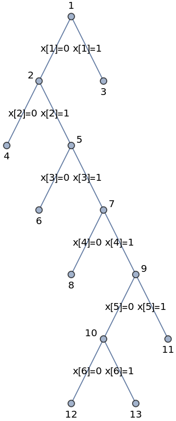
The 0-1 KNAPSACK PROBLEM
The 0-1 KNAPSACK PROBLEM
The 0-1 knapsack problem, which restricts the number of copies of each kind of item to zero or one. Given a set of items numbered from 1 up to, each with a weight and a value , along with a maximum weight capacity,
maximize ∑ p[i] x[i]
subject to ∑ ci[] x[i] ⩽ C and x[i] belongs {1,2,...,n}
Here represents the number of instances of item to include in the knapsack. Informally, the problem is to maximize the sum of the values of the items in the knapsack so that the sum of the weights is less than or equal to the knapsack's capacity.
Check accuracy of the Greedy Algorithm on the Fractional Knapsack problem with the Wolfram Language
Check accuracy of the Greedy Algorithm on the Fractional Knapsack problem with the Wolfram Language
In[]:=
Maximize[ ( 7x1 + 9x2+5x3+8x4 +6x5+5x6), {3x1 + 4 x2+x3+3x4 +5x5+2x6 ≤ 10, x1 + x2 ≤ 1,x1 + x6 ≤ 1 ,x2 + x3 ≤ 1,x3 + x4 ≤ 1 ,x3 + x6 ≤ 1,x4 + x5 ≤ 1,x5 + x6 ≤ 1 , x1 ≥ 0, x2 ≥ 0,x3 ≥ 0,x4 ≥ 0,x5 ≥ 0,x6 ≥ 0}, {x1,x2,x3,x4,x5,x6},Integers]
Out[]=
{22,{x10,x21,x30,x41,x50,x61}}
In[]:=
benefits={7,9,5,8,6,5}; weights={3,4,1,3,5,2};vars=Table[Subscript[x,s],{s,6}]
Out[]=
{,,,,,}
x
1
x
2
x
3
x
4
x
5
x
6
In[]:=
obj=benefits.vars
Out[]=
7+9+5+8+6+5
x
1
x
2
x
3
x
4
x
5
x
6
In[]:=
constr1=weights.vars≤10constr2=Subscript[ x,1]+Subscript[x,2]≤1constr3= Subscript[ x,1]+Subscript[x,6]≤1constr4=Subscript[ x,2]+Subscript[x,3]≤1constr5= Subscript[ x,3]+Subscript[x,4]≤1constr6=Subscript[ x,3]+Subscript[x,6]≤1constr7=Subscript[ x,4]+Subscript[x,5]≤1constr2= Subscript[ x,5]+Subscript[x,6]≤1
Out[]=
3+4++3+5+2≤10
x
1
x
2
x
3
x
4
x
5
x
6
Out[]=
x
1
x
2
Out[]=
x
1
x
6
In this section, we are able to test variety of the Mathematica already made commands to see how well our proposed Fractional Knapsack model works
Conclusion
Conclusion
The adoption of our proposed model and algorithm (Fractional Knapsack Algorithm) and it is first of its kind that will be on the Mathematica Repository. It gave an optimal allocation of resource to the projects in the district. It enabled a cut down of the number of uncompleted projects in the district. The selected projects were also able to be executed and completed within the available budget constraint. Because of the optimal operational resource, the projects were able to be executed at a minimal cost without exceeding the budgeted allocation. The decision procedures for allocation of projects would go a long way in solving the problem of indiscriminate allocation of projects by decision makers, since it would select only the feasible projects that can be executed and completed within the allocated budgetary at optimal cost and reduce the high rate of uncompleted projects in the district. The algorithm would provide optimal benefit, reduce cost of project execution and ensure that all selected projects are completed. The algorithm can be successfully applied to project management problem across the districts in other part of the country.