In this project we build a multiway graph for the two-dimensional Ising model. We compute the energies for each configuration. We try different rules to generate configurations of the system, which creates new multiway graphs. We look at loops in a multiway graph, given an evolution function some states can only reach some of the other states, and in general there would be multiple connected components in the graph, loops, stable states, etc. This project can be extended to the Potts model.
Introduction
Introduction
We begin our analysis by calculating the energy of the Ising model for the two-dimensional case. We will write functions to generate the two-dimensional Ising configurations, calculate the energy and magnetization.
In[]:=
Config2D[numberofspins_]:=Tuples[{1,-1},{numberofspins,numberofspins}];Magnetization2D[numberofspins_]:=Apply[Plus,#,{0,1}]&/@Config2D[numberofspins];Energy1[M_]:=Block[{s=Dimensions[M][[1]]},ParallelTable[(-1/2)*M[[i,j]]*(M[[Mod[i+1,s,1],j]]+M[[Mod[i-1,s,1],j]]+M[[i,Mod[j+1,s,1]]]+M[[i,Mod[j-1,s,1]]]),{i,1,s},{j,1,s}]];EnergyTotal[numberofspins_]:=Total[Total[Energy1[#]&/@Config2D[numberofspins],{3,3}],{2}]
The energy function, although correct, is slower than the one in “A New Kind of Science”, so we will use that one later on.
In[]:=
Energy2D[config_]:=-1/2Total[configListConvolve[{{0,1,0},{1,0,1},{0,1,0}},config,2],2];Energy2DTotal[s_]:=-1/2Total[#ListConvolve[{{0,1,0},{1,0,1},{0,1,0}},#,2],2]&/@Config2D[s];
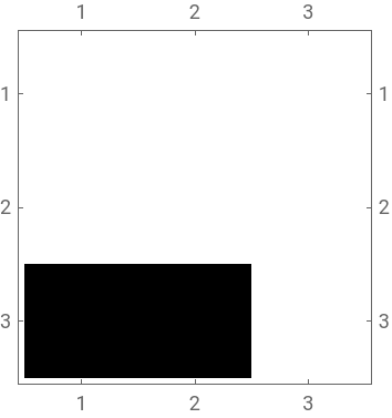
We now verify that the configuration function of the Ising model works correctly for the two-dimensional case.
In[]:=
MatrixForm/@Config2D[3]//Length
Out[]=
512
In[]:=
MatrixPlot[Config2D[3][[7]],ColorRules->{1White,-1Black}]
In[]:=
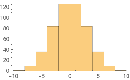
Histogram[Magnetization2D[3],{"Raw",Length[Counts[Magnetization2D[3]]]}]
In[]:=
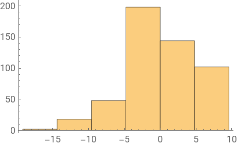
Histogram[Energy2DTotal[3],{"Raw",Length[Counts[Energy2DTotal[3]]]}]
Out[]=
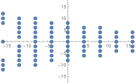
Let us plot the energy dependence on magnetization as in “A New Kind of Science” only for the two-dimensional case
In[]:=
ListPlot[Thread[{Energy2DTotal[4],Magnetization2D[4]}],PlotStylePointSize[Large]]
In[]:=
ListPlot[Thread[{Energy2DTotal[3],Magnetization2D[3]}],PlotStylePointSize[Large]]
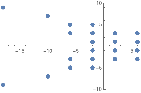
First attempt: rules of system evolution (spin-flip and spin-exchange)
First attempt: rules of system evolution (spin-flip and spin-exchange)
First, we decided to try spin-flip and spin-swapping rules. Despite the fact that they gave interesting results and closed cycles inside the graph, it was not possible to build all statistics from such rules automatically. Despite the fact that they gave interesting results and closed cycles inside the graph, it was not possible to build all statistics automatically from such rules.
In[]:=
MatrixForm/@ReplaceList[Config2D[3][[7]],{{x___,{y___,z_,h___},j___}:>{x,{y,-z,h},j}}]
Out[]=
,
,
,
,
,
,
,
,
-1 | 1 | 1 |
1 | 1 | 1 |
-1 | -1 | 1 |
1 | -1 | 1 |
1 | 1 | 1 |
-1 | -1 | 1 |
1 | 1 | -1 |
1 | 1 | 1 |
-1 | -1 | 1 |
1 | 1 | 1 |
-1 | 1 | 1 |
-1 | -1 | 1 |
1 | 1 | 1 |
1 | -1 | 1 |
-1 | -1 | 1 |
1 | 1 | 1 |
1 | 1 | -1 |
-1 | -1 | 1 |
1 | 1 | 1 |
1 | 1 | 1 |
1 | -1 | 1 |
1 | 1 | 1 |
1 | 1 | 1 |
-1 | 1 | 1 |
1 | 1 | 1 |
1 | 1 | 1 |
-1 | -1 | -1 |
In[]:=
EvolutionFuncSF[list_]:=ReplaceList[list,{{x___,{y___,z_,h___},j___}:>{x,{y,-z,h},j}}];EvolutionFuncSF1[list_]:=ReplaceList[list,{{x__,{y___,z_,h___},j__}:>{-j,{y,-z,h},x}}];EvolutionFuncSF2[list_]:=ReplaceList[list,{{x__,{y___,z_,h___},j__}:>{j,{y,-z,h},x}}];EvolutionFuncSF3[list_]:=ReplaceList[list,{{s___,x__,{y___,z_,h___},j__,d___}:>{d,j,{y,-z,h},x,s}}];
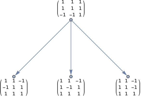
The actions of the rules can be visualized as follows:
In[]:=
NestGraph[EvolutionFuncSF1,{Config2D[3][[7]]},1,VertexLabels->Automatic,GraphLayout->"LayeredEmbedding"]
In[]:=
graphSF=NestGraph[EvolutionFuncSF,Config2D[3],1,VertexShapeFunction->Function[Inset[ArrayPlot[#2,ColorRules->{-1->White,1->Black},ImageSize->20,PlotLabel->Energy2D[#2]],#1,#3]],PerformanceGoal->"Quality",(*GraphLayout->"LayeredDigraphEmbedding",*)AspectRatio->1/2]
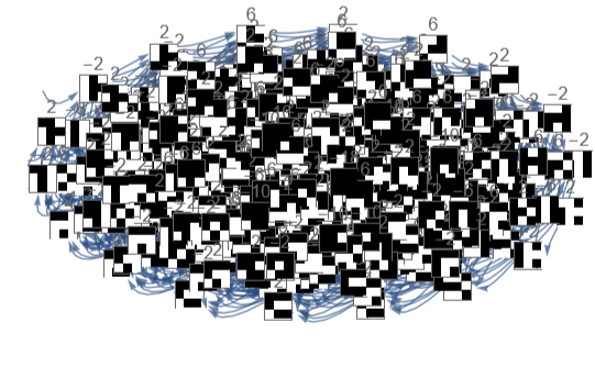
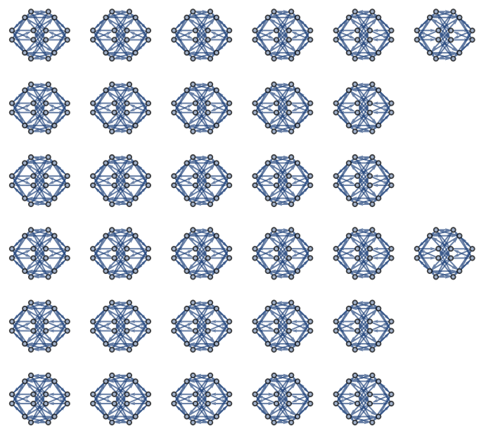
Here we have constructed a multiway graph with one of the evolution rules defined above . The vertices of the graph are graphical configurations of the Ising model with energies . In this form the graph is not so informative, so we investigate the connected components.
In[]:=
graphSF1=NestGraph[EvolutionFuncSF1,Config2D[3],10]
In[]:=
graphSF2=NestGraph[EvolutionFuncSF2,Config2D[3],10];graphSF3=NestGraph[EvolutionFuncSF3,Config2D[3],10];
In[]:=
GraphDistanceMatrix[graphSF]//MatrixPlot
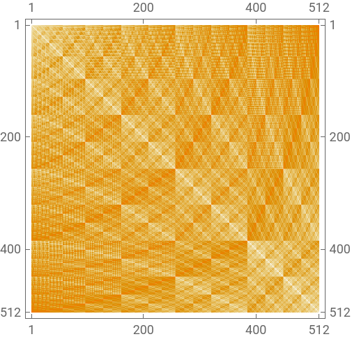
As we can see, in the first graph the shortest paths from vertex to vertex will be finite, while in the other graphs there are infinities . This means that some of the vertices are not connected to each other, the graph decomposes into unconnected subgraphs.
Let us consider the cycle energies of each subgraph. For the first graph we did not calculate, since it is a complete graph.
In the remaining three graphs, the energy in the subgraphs is not conserved, so we proceed to the second attempt .
Second attempt: rules of system evolution (Cellular Automaton for 1D)
Second attempt: rules of system evolution (Cellular Automaton for 1D)
The trick for creating this rule is to turn a two-dimensional system into a one-dimensional system, and then apply the CellularAutomaton function to the one-dimensional chain of spins. As it turned out, this was the wrong way to do it, because evolution happens in a one-dimensional system, and we need evolution in a two-dimensional system. However, we decided to include this part because research is not always a linear process.
In this evolution, it was found that some rules for one-dimensional systems conserve energy during the evolution of certain two-dimensional states. These rules can be seen below.
Here we collect all the rules with cycles with energy conservation.
As we can see, not all rules that conserve energy in the one-dimensional case also conserve energy in the two-dimensional case. Moreover, only one rule 51 preserves energy for all states, the rules from the RulesEnergyPreserv array preserve energy only for some states.
It is interesting to compute if there are rules that preserve the entropy within a subgraph or completely for the whole graph. The procedure is almost the same.
This means that the rules that preserve energy also preserve entropy.
We can see that only one rule 51 preserves entropy for all states, the rules from the RulesEntropyPreserv array preserve entropy and energy only for some states.
Third attempt: rules of system evolution (Cellular Automaton for 2D)
Third attempt: rules of system evolution (Cellular Automaton for 2D)
Now, we come to the case where the cellular automaton is applied to a two-dimensional array. There are many 2D general rules:
The number of such rules is huge, so it is not possible to build statistics on all rules, as we did for 1D rules. Therefore, we will randomly select some of them and look at the energy.
Here we collect all the rules with cycles with energy and entropy conservation.
This means that the rules that preserve energy also preserve entropy.
Among the rules we have chosen, there are no rules that preserve energy and entropy for all states.
Concluding remarks
Concluding remarks
In summary, this project focused on the study of the 2D Ising model, exploring three different types of evolutionary rules. The initial rules involving spin-flip and spin-exchange were found to be more difficult to build statistics with. As an alternative approach, 1D Cellular Automaton based rules were used, although this is not an ideal way to implement Cellular Automaton in 2D systems. However, this approach provided interesting dynamics.
Through the investigation, it was discovered that for Cellular Automaton based rules in 1D systems, there exists a single rule that preserves both energy and entropy for each state in the system. In addition, specific rules were identified that conserved energy and entropy within subgraphs for certain states. Furthermore, when applying the same analysis and framework to the rules based on the 2D Cellular Automaton for 2D systems, it was discovered that the rules that preserve energy for some states also preserve entropy.
There are two possible directions for further development. First, we could explore more rules based on the 2D Cellular Automaton to improve the understanding of the dynamics of the system and the statistics. Second, the same analysis and framework can be applied to the Potts model, which includes more degrees of freedom, thus broadening the scope of the study. These future efforts have the potential to deepen our understanding of complex systems and their multiway evolutionary behavior.
Key words
Key words
◼
Ising Model
◼
Cellular Automata
◼
Multiway Systems
Acknowledgment
Acknowledgment
I would like to acknowledge my mentors Manojna Namuduri and Nikolay Murzin for their support and encouragement during the course of this project. I also would like to express my gratitude to Xerxes Arsiwalla for useful discussions and guidance, and the organizers for giving me this opportunity. Finally, I thank Stephen Wolfram for defining this interesting project for me.
References
References
CITE THIS NOTEBOOK
CITE THIS NOTEBOOK
Multiway systems for exactly solved lattice models
by Aisel Shiralieva
Wolfram Community, STAFF PICKS, 13 July, 2023
https://community.wolfram.com/groups/-/m/t/2960072
by Aisel Shiralieva
Wolfram Community, STAFF PICKS, 13 July, 2023
https://community.wolfram.com/groups/-/m/t/2960072