Climate and weather datasets form the backbone of Earth observation science. Google Earth Engine hosts decades of satellite-derived temperature, precipitation, atmospheric, and radiation products at global scales. This chapter demonstrates how to extract, process, and analyze these datasets using the GoogleEarthEngineClient paclet alongside Wolfram Language's built-in statistical and time series tools.
Every example follows a consistent pattern: build a server-side processing pipeline with the operator, retrieve the result with , , or , then analyze client-side with Wolfram Language functions such as , , , and .
Every example follows a consistent pattern: build a server-side processing pipeline with the
//
GEECompute
GEEIdentify
GEEComputePixels
TimeSeries
LinearModelFit
MovingAverage
DateListPlot
Prerequisite:
se of this paclet is subject to the Google Earth Engine Terms of Service.
Authenticate per Google Earth Engine (GEE) client paclet, Section 1.3
and then load the paclet with.
se of this paclet is subject to the Google Earth Engine Terms of Service.
Authenticate per Google Earth Engine (GEE) client paclet, Section 1.3
and then load the paclet with
Needs["DiegoZviovich`GEE`"]
3.1 Surface Temperature
Land surface temperature (LST) is a fundamental climate variable that governs surface energy balance, evapotranspiration, and urban comfort. Two complementary satellite products provide LST at different spatial and temporal resolutions.
3.1.1 MODIS Land Surface Temperature
3.1.1 MODIS Land Surface Temperature
The product delivers 8-day composite LST at 1 km resolution. Raw pixel values are stored as scaled integers; multiply by 0.02 to convert to Kelvin, then subtract 273.15 to obtain degrees Celsius.
MODIS/061/MOD11A2
Map daytime LST over a city to reveal the urban heat island effect:
In[]:=
(*BuildasummerLSTcompositeforPhoenix,Arizona*)loc=GeoCircle,Quantity[50,"Kilometers"];lstExpr=GEECollection["MODIS/061/MOD11A2"]//GEEFilterDate["2024-06-01","2024-09-01"]//GEEFilterBounds[loc]//GEESelectBands[{"LST_Day_1km"}]//GEEMean//GEEMultiply[0.02]//GEEAdd[-273.15];(*Renderasacolor-mappedtemperatureimage*)lstImage=GEEComputePixels[loc,lstExpr,"VisParams"-><|"min"->35,"max"->55,"palette"->{"#2166ac","#67a9cf","#d1e5f0","#fddbc7","#ef8a62","#b2182b"}|>,"ImageSize"->{512,512}](*Blue=coolerparksandirrigatedareas,red=hotimpervioussurfaces*)
Out[]=
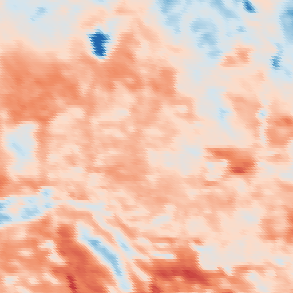
The scale factor pipeline () runs entirely server-side, so you receive physically meaningful Celsius values without downloading raw integers.
GEEMultiply[0.02] // GEEAdd[-273.15]
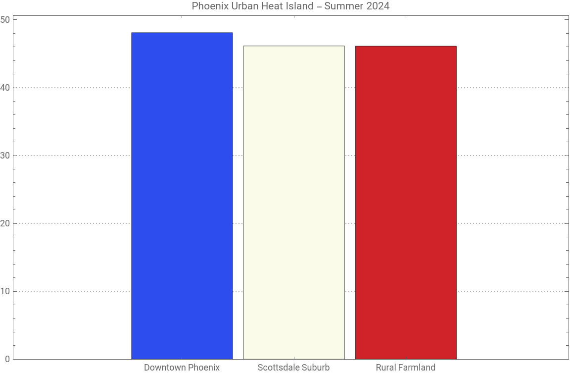
Query LST at specific points across the urban-rural gradient:
In[]:=
(*Definepoints:downtown,suburb,agriculturalfringe*)points=<|"Downtown Phoenix"->GeoPosition[{33.45,-112.07}],"Scottsdale Suburb"->GeoPosition[{33.50,-111.93}],"Rural Farmland"->GeoPosition[{33.38,-112.25}]|>;lstResults=Association@KeyValueMap[Function[{name,pos},name->GEEIdentify[pos,lstExpr]["Values"][[1]]],points];BarChart[lstResults,ChartLabels->Keys[lstResults],AxesLabel->{None,"LST (°C)"},PlotLabel->"Phoenix Urban Heat Island - Summer 2024",ChartStyle->"TemperatureMap",ImageSize->Large,PlotTheme->"Detailed"](*Downtowntypically5-10°Cwarmerthansurroundingfarmland*)
Out[]=
3.1.2 Landsat Thermal Band
3.1.2 Landsat Thermal Band
Landsat 8 Collection 2 Level 2 provides surface temperature via the band at 30 m resolution -- much finer than MODIS. This enables intra-urban thermal comparisons between parks and built-up areas. For the Landsat thermal scale factors and band conventions, see Section 2.2. For urban heat island analysis using these thermal products, see Section 7.2.
ST_B10
Compare LST between an urban park and its surroundings:
In[]:=
(*Cloud-filteredLandsat8surfacetemperatureforAustin,TX*)landsatLST=GEECollection["LANDSAT/LC08/C02/T1_L2"]//GEEFilterDate["2024-06-01","2024-09-01"]//GEEFilterBounds[{-97.8,30.2,-97.7,30.35}]//GEEFilterProperty["CLOUD_COVER","LessThan",20]//GEESelectBands[{"ST_B10"}]//GEEMedian//GEEMultiply[0.00341802]//GEEAdd[149.0-273.15];(*Sampleatmultiplepoints:ZilkerParkvs.downtown*)parkPoints={GeoPosition[{30.267,-97.773}],(*ZilkerParkcenter*)GeoPosition[{30.271,-97.770}],(*ZilkerParkedge*)GeoPosition[{30.264,-97.776}](*BartonSprings*)};urbanPoints={GeoPosition[{30.267,-97.743}],(*CongressAvenue*)GeoPosition[{30.270,-97.740}],(*East6thStreet*)GeoPosition[{30.265,-97.747}](*RaineyStreet*)};parkTemps=Mean[First/@(#["Values"]&/@GEEGetSamples[parkPoints,landsatLST])];urbanTemps=Mean[First/@(#["Values"]&/@GEEGetSamples[urbanPoints,landsatLST])];Grid[{{"Location","Mean LST (°C)"},{"Zilker Park",Round[parkTemps,0.1]},{"Downtown",Round[urbanTemps,0.1]},{"Difference",Round[urbanTemps-parkTemps,0.1]}},Frame->All]
3.1.3 Satellite vs. Ground Station Validation
3.1.3 Satellite vs. Ground Station Validation
Comparing satellite-derived LST with ground-based air temperature helps establish confidence in the remote sensing product. Note that LST (skin temperature) and air temperature (measured at ~2 m height) differ physically, so systematic offsets are expected.
3.2 Precipitation and Rainfall
Precipitation is the primary driver of hydrology, agriculture, and flood risk. Two complementary products provide global coverage at different resolutions.
3.2.1 CHIRPS Daily Rainfall
3.2.1 CHIRPS Daily Rainfall
Monthly rainfall accumulation:
Rainfall anomaly -- compare to the long-term mean:
A rainfall anomaly highlights whether a given month was wetter or drier than normal. Compute the long-term July mean (e.g., 2010-2023), then subtract from the current year.
Note: This simplified approach averages all daily values in the date range, not just July values. For a precise July climatology, compute each year's July total separately and average them (see Section 3.2.3 for the per-month loop pattern).
3.2.2 GPM IMERG Precipitation
3.2.2 GPM IMERG Precipitation
3.2.3 Monthly Rainfall Time Series with Trend Analysis
3.2.3 Monthly Rainfall Time Series with Trend Analysis
Building a multi-month rainfall time series from GEE point queries and analyzing it with Wolfram Language statistical tools is a powerful workflow for detecting climate trends.
Apply smoothing and trend detection:
3.3 Atmospheric Data
Atmospheric reanalysis products combine satellite observations with numerical weather models to produce spatially complete, temporally consistent records of key atmospheric variables.
3.3.1 ERA5-Land Reanalysis
3.3.1 ERA5-Land Reanalysis
Extract a temperature time series for a single point over one year:
Wind speed map from u and v components:
Wind speed is not stored directly in ERA5; instead, the eastward (u10) and northward (v10) components are provided separately. Wind speed is the magnitude of the wind vector: sqrt(u^2 + v^2). The following example computes this entirely server-side using expression builder arithmetic.
3.3.2 An Alternative Approach: GEEExpression for Wind Speed
3.3.2 An Alternative Approach: GEEExpression for Wind Speed
3.3.3 MODIS Aerosol Optical Depth
3.3.3 MODIS Aerosol Optical Depth
Query AOD at specific cities for comparison:
3.4 Evapotranspiration
Evapotranspiration (ET) quantifies water loss from the land surface through soil evaporation and plant transpiration. It is a critical variable for agricultural water management, drought assessment, and hydrological modeling. For a complete watershed-scale water budget combining precipitation and ET, see Section 6.8.
3.4.1 MODIS Evapotranspiration
3.4.1 MODIS Evapotranspiration
Map seasonal ET over an agricultural region:
3.4.2 Irrigated vs. Rainfed Cropland ET Comparison
3.4.2 Irrigated vs. Rainfed Cropland ET Comparison
3.4.3 Water Balance: Precipitation Minus Evapotranspiration
3.4.3 Water Balance: Precipitation Minus Evapotranspiration
A simplified water balance model uses precipitation minus ET to estimate net water availability. Positive values indicate surplus (potential runoff or groundwater recharge); negative values indicate deficit (requiring irrigation or drawing from storage).
3.5 Multi-Year Climate Analysis
Longer time horizons reveal trends, periodicities, and climate shifts that single-year snapshots cannot capture. This section demonstrates decadal analysis workflows that combine GEE data extraction with Wolfram Language statistical and time series functions.
3.5.1 Decadal Temperature Trend
3.5.1 Decadal Temperature Trend
Extract annual mean land surface temperature for 10 years, fit a linear trend, and forecast future values.
3.5.2 Time Series Forecasting
3.5.2 Time Series Forecasting
3.5.3 Drought Monitoring with Standardized Precipitation Index
3.5.3 Drought Monitoring with Standardized Precipitation Index
The Standardized Precipitation Index (SPI) transforms precipitation data into a standardized metric where negative values indicate drought. This simplified implementation computes monthly precipitation z-scores using the long-term mean and standard deviation.
3.5.4 Detecting Seasonal Cycles with Fourier Analysis
3.5.4 Detecting Seasonal Cycles with Fourier Analysis
3.6 Solar Radiation
Solar radiation drives the surface energy budget and is critical for solar energy site assessment. Combining Wolfram Language's astronomical functions with GEE terrain data enables physically based irradiance estimation.
3.6.1 Solar Geometry with Wolfram Language
3.6.1 Solar Geometry with Wolfram Language
3.6.2 Terrain-Adjusted Solar Irradiance
3.6.2 Terrain-Adjusted Solar Irradiance
Slope and aspect from GEE terrain data determine how a surface is oriented relative to incoming sunlight. South-facing slopes in the Northern Hemisphere receive more direct radiation than north-facing slopes.
Estimate clear-sky solar irradiance on a tilted surface:
3.6.3 Hillshade Visualization
3.6.3 Hillshade Visualization
3.7 Putting It All Together: Multi-Variable Climate Dashboard
This final section demonstrates how to combine multiple climate variables into a unified analysis. The workflow extracts temperature, precipitation, ET, and wind data for a single region and present them as an integrated dashboard.
Compute annual summary statistics:
Summary
Quick Reference: Datasets Used in This Chapter
Quick Reference: Key Functions Used in This Chapter
CITE THIS NOTEBOOK
CITE THIS NOTEBOOK
Google Earth Engine (GEE) paclet: climate and weather analysis
by Diego Zviovich
Wolfram Community, STAFF PICKS, May 16, 2026
https://community.wolfram.com/groups/-/m/t/3716885
by Diego Zviovich
Wolfram Community, STAFF PICKS, May 16, 2026
https://community.wolfram.com/groups/-/m/t/3716885