Checking the preservation of the Schwarzschild metric in a Graph Evolution
Roberto Caiozzo
University of Amsterdam
Roberto Caiozzo
University of Amsterdam
This projects offers a preliminary approach on how to check wether the iterative application of a specific graph evolution rule preserves a 2D Schwarzschild metric. This is done by analysing the area relationship to the radius of circles on the evolved graph surface, which can show dimensional or curvature deviation in the geometry of the Graph. While still very approximative this method could easily be abstracted to n-dimensional space by using the radius relationship of the volume of an n-sphere.
This projects offers a preliminary approach on how to check wether the iterative application of a specific graph evolution rule preserves a 2D Schwarzschild metric. This is done by analysing the area relationship to the radius of circles on the evolved graph surface, which can show dimensional or curvature deviation in the geometry of the Graph. While still very approximative this method could easily be abstracted to n-dimensional space by using the radius relationship of the volume of an n-sphere.
Main Project
Main Project
We start by plotting a Flamm's paraboloid, a visualization of the 2D static spacetime curvature of a Schwarzschild solution. It is useful because it preserves the distances of the metric but it should not be used to analyze a particle's geodesics given that all possible paths are spacelike within the graph [1].
Given that we are only interested in the metric preservation and not in the particles' geodesics this is a good enough approximation of the a Schwarzschild solution for the purposes of the project. We use a Schwarzschild of 1 to simplify the calculations given that it does not impact the geometry.
Given that we are only interested in the metric preservation and not in the particles' geodesics this is a good enough approximation of the a Schwarzschild solution for the purposes of the project. We use a Schwarzschild of 1 to simplify the calculations given that it does not impact the geometry.
Plot3D[func=2Sqrt[Sqrt[x^2+y^2]-1],{x,-5,5},{y,-5,5},PlotStyleDirective[Opacity[0.8],Black,Specularity[Gray,50]]]
(Debug) Out[]=

Plot3D[func=2Sqrt[Sqrt[x^2+y^2]-1],{x,-100,100},{y,-100,100},PlotStyleDirective[Opacity[0.8],Black,Specularity[Gray,50]]]
(Debug) Out[]=

We can then use the CurvedManifoldToGraph functions to randomly sprinkle on the paraboloid nodes connected with edge relations depending on distance between the nodes on paraboloid. The discreteness and number of points must be chosen in such a way that all points should be connected by at least one geodesic but not to an excessive number of other nodes, this is to preserve the physical properties of space within the Graph. Computational cost should also be considered when using high amounts of nodes, as a higher amount of nodes will cause a exponential growth to the number of computations necessary to implement successive rules to the graph.
Down is a 3D representation of an example of a graph generated through this method.
Down is a 3D representation of an example of a graph generated through this method.
blackhole:=2Re[Sqrt[Sqrt[x^2+y^2]]-1]-z==0manifold=ResourceFunction["ExtrinsicCurvedManifoldToGraph"][blackhole,{x,y,z},{{-5,5},{-5,5},{-5,5}},5.5,20]graph=manifold["SpatialGraph"]
(Debug) Out[]=
ManifoldGraph


(Debug) Out[]=

We can then extract the graph as a list and then apply a rule iteratively to it through the WolframModel function. The main limitation when you are extracting the list is that given that the edges are non directional in the sprinkled graph, therefore we must arbitrarily choose a n-relationship to subdivide the graph in, and arbitrarily decide the direction of the edges. In this case I picked binary relations and made it so for each edge in the graph the extracted list has two edges, one for each direction.
Down is an example taking a random 2_2 -> 2_2, 2_2 rule to ensure the expansion of the graph and iterating it 3 times over the graph.
Down is an example taking a random 2_2 -> 2_2, 2_2 rule to ensure the expansion of the graph and iterating it 3 times over the graph.
matr=AdjacencyMatrix[graph]hyperlist:={}For[i=1,i≤Part[Dimensions[matr],1],i++,For[j=1,j≤Part[Dimensions[matr],2],j++,If[Part[matr,i,j]1,AppendTo[hyperlist,{i,j}],Nothing]]]final:=ResourceFunction["WolframModel"][{{x,y}}{{x,y},{y,z}},hyperlist,3,"FinalState"]ResourceFunction["WolframModel"][{{x,y}}{{x,y},{y,z}},final,0,"FinalStatePlot"]
(Debug) Out[]=
SparseArray

(Debug) Out[]=
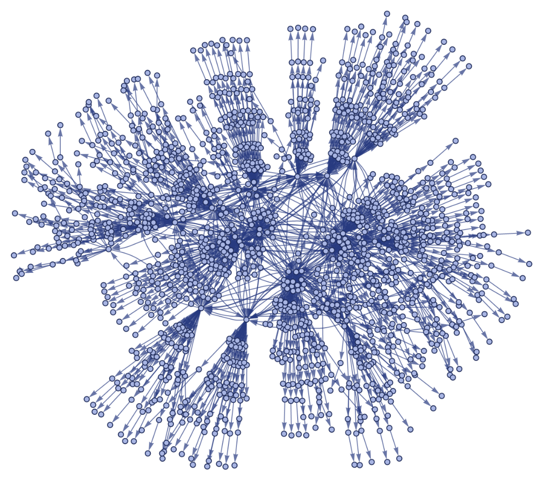
We can then analyse this final graph using the properties of n-balls on curved n-dimensional space to check wether the geometry of the Schwarzschild
solution is preserved. In a Euclidian continuous geometrical space the volume of an n-ball will be of the form [3]
We can then analyse this final graph using the properties of n-balls on curved n-dimensional space to check wether the geometry of the Schwarzschild
solution is preserved. In a Euclidian continuous geometrical space the volume of an n-ball will be of the form [3]
V(r)=
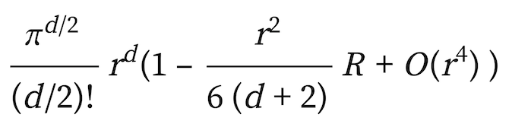
Where R is the Ricci curvature scalar of the metric and d is the dimension of the space. In our discrete version there will be different coefficients and more influences of lower order r, however the leading terms will likely stay the same to the function above. In a Schwarzschild metric the Ricci Scalar is zero everywhere outside the singularity, and if the geometry is preserved by the rule at the very list the dimensionality and curvature of the graph should stay the same [2]. This means that a good initial filter for rules that preserve the metric of the graph will be rules where in the evolved graph V_r ~ r^2.
where r is defined as the number of edges between two points and V_r is defined as the number of points which can be reached by a radius r from the origin. To check for this we extract 10 random points (to account for potential local distortions due to boundary effects) and use the HypergraphNeighborhoodVolumes function to obtain the value of the Areas for all possible radiuses for all the chosen points. We can then fit a parabola to the datapoints and check if the relationship holds up (ignoring low and high radiuses points due to discreteness and boundary effects respectively).
where r is defined as the number of edges between two points and V_r is defined as the number of points which can be reached by a radius r from the origin. To check for this we extract 10 random points (to account for potential local distortions due to boundary effects) and use the HypergraphNeighborhoodVolumes function to obtain the value of the Areas for all possible radiuses for all the chosen points. We can then fit a parabola to the datapoints and check if the relationship holds up (ignoring low and high radiuses points due to discreteness and boundary effects respectively).
assoc=ResourceFunction["HypergraphNeighborhoodVolumes"][final,"Random"10]keylist=Keys[assoc]shortestmaxradius=Length[assoc[Part[keylist,1]]]For[i=1,i≤10,i++,If[Length[assoc[Part[keylist,i]]]<shortestmaxradius,shortestmaxradius=Length[assoc[Part[keylist,i]]],shortestmaxradius=shortestmaxradius]]Dataplot:={{0,0}}For[j=1,j≤10,j++,For[i=2,i≤shortestmaxradius,i++,AppendTo[Dataplot,{i-1,Part[assoc[Part[keylist,j]],i]}]]]parabola=Fit[Dataplot,{x^2},x]Show[ListPlot[Dataplot,PlotStyleRed],Plot[parabola,{x,0,shortestmaxradius}]]
(Debug) Out[]=
101{1,4,52,545,1160,1470,1529,1532},109{1,4,20,176,738,1284,1505,1532},306{1,3,5,60,624,1243,1503,1532},376{1,3,5,60,624,1243,1503,1532},536{1,3,5,48,455,1069,1438,1528,1532},595{1,3,14,115,563,1146,1465,1532},662{1,3,5,32,318,912,1367,1518,1532},843{1,2,4,28,272,896,1382,1528,1532},1034{1,2,3,50,544,1160,1470,1529,1532},1455{1,2,4,64,633,1250,1505,1532}
(Debug) Out[]=
{101,109,306,376,536,595,662,843,1034,1455}
(Debug) Out[]=
8
(Debug) Out[]=
35.8274
2
x
The closer the fitted parabola is to the datapoints the more the metric is preserved, as we can see in the image below the data can be fitted much better with a function depending on r^3 (as shown by the green function) indicating that the metric is likely not preserved (it is important to remember that the last few radius points are less important due to boundary distortion effects. However, a much bigger graph with larger possible radiuses would probably offer a more definitive conclusion, this was however the computational limit of my computer.
Conclusions
Conclusions
The main issues with this project are the high computational load and the possible issues with the distortion caused by the Random picking of points on the edges of the graph or near the Schwarzschild radius. Moreover this is far from a concrete filter, it's just a first screening for Rules that clearly do not preserve the metric and still needs a lot of work before it becomes an automatic iterative function. Two easy ways for this filter to break are when the Ricci curvature and dimension change in conjunction and when the Schwarzschild metric is substituted by a different metric with the same Ricci scalar (e.g Minkowski space). Ideally an improved version of this method could be used to analyse multiple rules in a row with a higher accuracy and more datapoints, however the computational costs might be hard to remove. If this was achieved it could actually allow to help in the search of rules which are able to simulate systems involving a Schwarzschild spacetime like black holes and other simplified star systems.
Keywords
Keywords
◼
Schwarzschild metric
◼
Flamm’s paraboloid
◼
Wolfram Model
Acknowledgment
Acknowledgment
Mentor: Tobias Canavesi
I want to thank my mentor Tobias for helping me many times throughout this journey, Dr. Xerxes D. Arsiwalla for helping me understand how to extract information from the hypergraph and Dr. Jonathan Gorard and Dr. Stephen Wolfram for helping me with understanding how to approach the project and how the model relates to physics. In general I would also like to thank the whole Wolfram Physics Winter School for allowing for this great opportunity.
References
References
◼
[1] Chrusciel , Piotr T. Geometry of Black Holes, University of Vienna, July 2018, homepage.univie.ac.at/piotr.chrusciel/teaching/Black%20Holes/BlackHolesViennaJanuary2015.pdf.
◼
[2] Misner, Charles W., et al. Gravitation. Princeton University Press, 2017.
◼
[3] Wolfram, Stephen. “A Class of Models with the Potential to Represent Fundamental Physics.” Complex Systems, vol. 29, no. 2, 2020, pp. 107–536., doi:10.25088/complexsystems.29.2.107.