Line, Surface and Contour Integration
Line, Surface and Contour Integration
Another Milestone for Special Functions
Another Milestone for Special Functions
Finite Fields!
Finite Fields!
More, Stronger Computational Geometry
More, Stronger Computational Geometry
Visualizations Begin to Come Alive
Visualizations Begin to Come Alive
Visualizations Begin to Come Alive
This was one of my favorite things about 13.3. I don’t understand all the math stuff but this is something simple and helpful that I can use.
In[]:=
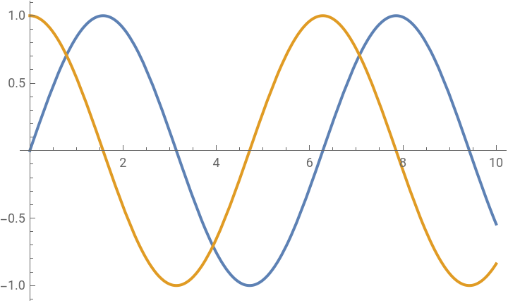
Plot[{Sin[x],Cos[x]},{x,0,10}]
Out[]=
In[]:=
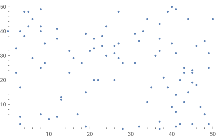
ListPlot[RandomInteger[50,{100,2}]]
Out[]=
In[]:=
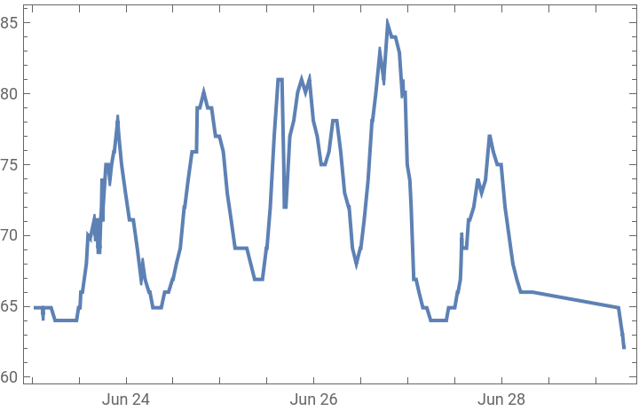
DateListPlot[AirTemperatureData[Today-,Today]]
Out[]=
In[]:=
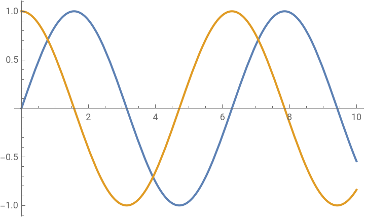
Plot[{Sin[x],Cos[x]},{x,0,10},PlotHighlighting->Directive[Red,Thickness[.02]]]
Out[]=
In[]:=
Plot[{Sin[x],Cos[x]},{x,0,10},PlotHighlighting->"XSlice"]
Out[]=
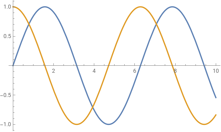
In[]:=
Plot[{Sin[x],Cos[x]},{x,0,10},PlotHighlighting->{{"XDropline",<|"Style"->Red|>},{"XAxisLabel",<|"LabelStyle"->13|>}}]
Out[]=
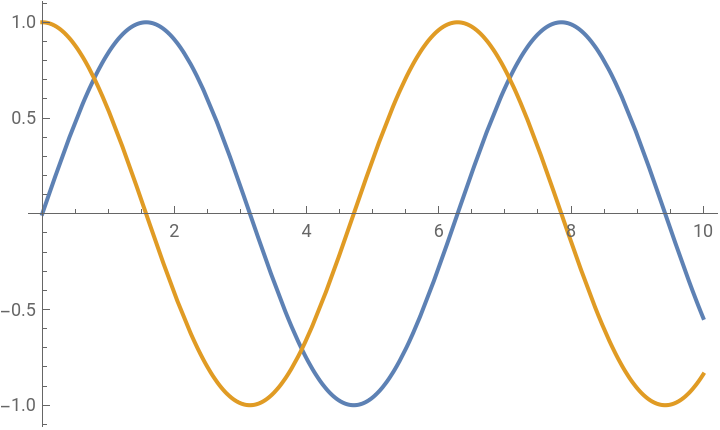
In[]:=
Plot[{x,-x,Highlighted[xSin[x],"Ball"]},{x,0,20}]
Out[]=
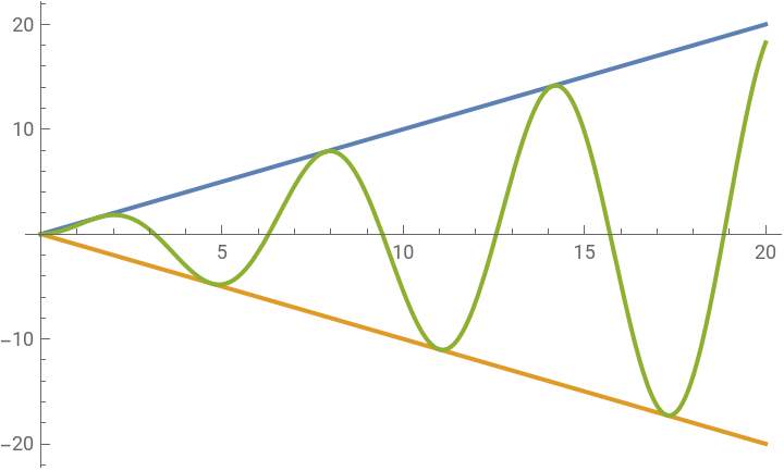
In[]:=
Plot[{x,-x,Highlighted[xSin[x],Placed["XAxisLabel",{Automatic,0}]]},{x,0,20}]
Out[]=
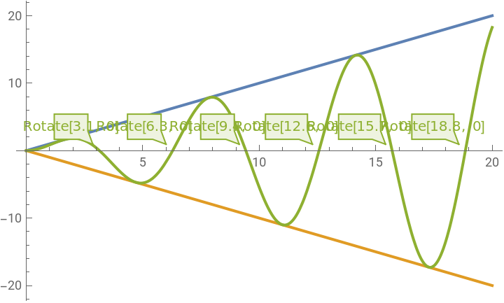
In[]:=
Plot[{x,-x,Style[xSin[x],Haloing[Red]]},{x,0,20}]
Out[]=
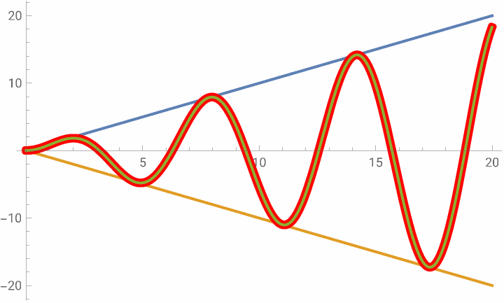
In[]:=
ListPlot[Table[Highlighted[RandomInteger[100,2],Haloing[RandomColor[]]],50]]
Out[]=
In[]:=
ListPlot[Table[Highlighted[RandomInteger[100,2]],50]]
Out[]=
I don’t really see any notable difference with and without Haloing.
Style country borders:
A colorful world map:
Publishing to Augmented + Virtual Reality
Publishing to Augmented + Virtual Reality
I guess I will have to wait for support for Windows.
Getting the Details Right: The Continuing Story
Getting the Details Right: The Continuing Story
I would like to note that FileDate does not support DateGranularity at the moment.
Even Easier to Type: Affordances for Wolfram Language Input
Even Easier to Type: Affordances for Wolfram Language Input
The Elegant Code Project
The Elegant Code Project