Sound classification can be a hard task, especially when sound samples have just little variations that can be imperceptible to the human ear. The use of machines, and recently machine learning models, has shown to be an effective approach on solving the problem of classifying sounds. In medicine, these applications can help to improve diagnoses and have been a topic of research in areas as cardiology and pneumonology. Recent innovations such as a convolutional neural network identifying COVID-19 coughs and the MIT AI model detecting asymptomatic COVID-19 infections using cough recordings show that is possible to identify COVID-19 patients just by the sound of their coughs. We want to reproduce their results, using a labeled COVID-19 open source cough sound dataset. Our approach was to construct a recurrent neural network and feed in preprocessed audio signals using “MFCC” feature extraction. This approach gave us an accuracy of around 86% which is similar to the results obtained on different published studies, even when our data was highly limited to 121 samples.
Exploring the cough sound data
Exploring the cough sound data
The data set, which can be found HERE, consists of 121 segmented samples of cough sounds in .mp3 format, the samples corresponding to each class are inside a different folder (“pos” folder and “neg” folder).
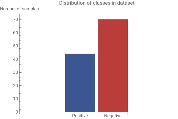
This data set has an small unbalance of classes, the 2 classes are distributed as follows:
◼
pos class: 48 samples positive for COVID-19 disease.
◼
neg class: 73 samples negative for COVID-19 disease.
The segmented data comes from 16 patients, so we have prepared the data in a way the test data folder wont contain audios of patients that are already in the train data folder
Define data directory:
In[]:=
dir="C:\\Users\\ECF0124A\\Downloads\\virufy_data-main\\clinical\\segmented";
Define a function that creates relation maps between the files and the corresponding labels:
In[]:=
loadFiles[dir_]:=Map[File[#]FileNameTake[#,{-2}]&,FileNames["*.mp3",dir,Infinity]];
Load the test and train data from the folder :
In[]:=
trainData=loadFiles[FileNameJoin[{dir,"train"}]];testData=loadFiles[FileNameJoin[{dir,"test"}]];
It is better if we make sure the data that feeds the model is randomized, in that way each batch on the training process will have equally class distributed data. We make sure the random appearance of the sample using the RandomSample Function:
In[]:=
trainDataRandom=loadFiles[FileNameJoin[{dir,"train"}]]//RandomSample;testDataRandom=loadFiles[FileNameJoin[{dir,"test"}]]//RandomSample;
Examine the first three elements of the data set:
In[]:=
trainDataRandom[[1;;3]]
Out[]=
Fileneg,Fileneg,Fileneg
As a last check we can hear the actual sound of the data selecting randomly one of the audios for the train set:
Play the audio for a train data point:
In[]:=
Audio[Keys[RandomChoice[trainDataRandom]]]
Out[]=
Class distribution
Class distribution
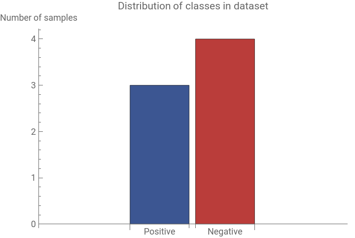
We can make a BarChart and observe the distribution of the two classes in study. There is an imbalance in sample sizes, but the difference is small enough that the model should still be effective.
In[]:=
BarChartCounts[Values[trainDataRandom]],
Out[]=
In[]:=
BarChartCounts[Values[testDataRandom]],
Out[]=
Create Audio MFCC Encoding
Create Audio MFCC Encoding
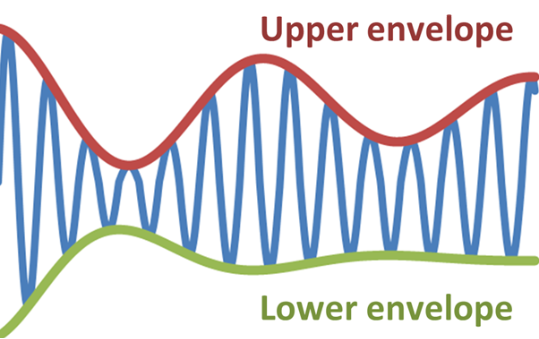
Audio encoding is an important step for audio classification, as any sound generated by humans is determined by the shape of their vocal tract (including tongue, teeth, etc). If this shape can be determined correctly, any sound produced can be accurately represented. The same happens with musical instruments -- even when two different instruments can be generating the same sound frequency, they will sound different because of the physical characteristics of the instrument (piano, guitar, flout, etc). The envelope of the time power spectrum of the speech signal is representative of the vocal tract, which MFCC accurately represents. Some diseases as a pulmonary disease, can affect the way the air travels through our respiratory system, so it may cause a difference in sound between a healthy patient and a sick patient.
MFCC or Mel Frequency Cepstral Coefficients was first introduced to characterize the seismic echoes resulting due to earthquakes. In order to obtain the Mel Frequency Cepstral Coefficients, we apply the Fourier Transform over the original sound wave on the time domain and then apply over the Fourier resulting spectrum the logarithm of the magnitude, finally applying a cosine transformation. This resulting spectrum, called the cepstrum in the quefrency domain, is neither in the frequency domain nor in the time domain.
We will use the “AudioMFCC” option on the NetEncoder function to make all this process automatic. We can choose also the amount coefficients we want on the result with the “NumberOfCoefficients” option.
Build the NetEncoder for an AudioMFCC feature extraction:
In[]:=
encoder=NetEncoder[{"AudioMFCC","TargetLength"All,"NumberOfCoefficients"40,"SampleRate"16000,"WindowSize"1024,"Offset"571,"Normalization""Max"}]
Out[]=
NetEncoder

Check the result of the AudioMFCC NetEncoder applied on a random audio sample. The output of the encoder is a rank-2 tensor of dimensions {n,nc}, where n is the number of partitions after the preprocessing is applied and nc is the number of coefficients used for the computation. We will show this with a MatrixPlot
In[]:=
encoder[Audio[RandomChoice[Keys[trainData]]]]//MatrixPlot
Out[]=
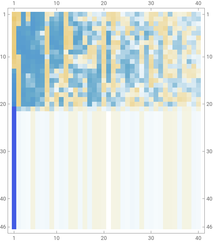
We can see how the audio has been converted into a matrix which represents the cepstral features of the audio, this will be the input of out model.
Build and train the model
Build and train the model
Recurrent Neural Networks (RNN)
Recurrent Neural Networks (RNN)
A recurrent neural network (RNN) is a class of artificial neural networks where connections between nodes form a directed graph along a temporal sequence. This allows it model temporal dynamic behavior, making them applicable to tasks such as handwriting recognition, video and movement classification or speech recognition.
We will build a recurrent neural network using the NetBidirectionalOperator and GatedRecurrentLayer, as well as LinearLayer, DropoutLayer and Ramp to add complexity to the network and avoid overfitting.
We will build a recurrent neural network using the NetBidirectionalOperator and GatedRecurrentLayer, as well as LinearLayer, DropoutLayer and Ramp to add complexity to the network and avoid overfitting.
◼
GatedRecurrentLayer: Gives the neural net the capacity of training over a sequence of coefficients instead of a one-by-one learning, this is usually done when the data has a sequence nature, as audio, video (sequence of images), and natural language (sequence of words).
◼
LinearLayer: Add neurons and complexity to the neural network.
◼
DropoutLayer: prevents overfitting by randomly turning off some of the neurons on the previous layer
Build the custom RNN
Build the custom RNN
We build a custom RNN which hyperparameters have been tuned by hand iterating them on a tune-train-evaluate process, that means:
1
.Choose a set of hyperparameters
2
.Train the model
3
. Evaluate the model
4
.Repeat steps 1,2 and 3
We repeat this process till the model shows low overfitting and high evaluation metrics, the result is the RNN we have below:
Create recurrent neural network with a 15 feature sequence, joined with a 16 neuron linear layer and dropout of 0.5 (for overfitting prevention). The output will be “pos” for COVID-19 disease and “neg” for the absence of COVID-19 disease:
Train the RNN
Train the RNN
Train the recurrent neural network over the train set and validates on the test set, this allow us to observe the training process and tune the hyperparameters of the network (amount of neurons on the LinearLayer, DropoutLayer number and GatedRecurrentLayer amount of features in sequence ).
Net evaluation
Net evaluation
After the training we will make an evaluation of the model, applying it to the previously unseen test data and measuring its performance. For that, we will try different metrics as:
◼
Accuracy: It is the ratio of correctly predicted observations to the total observations.
◼
F1 score: Is the weighted average of Precision and Recall
◼
Precision and recall: Precision is the ratio of correctly predicted positive observations to the total predicted positive observations while recall is the ratio of correctly predicted positive observations to the all observations in actual class (see an example on the image below).
◼
Confusion matrix plot: allows to see the true positive, true negative, false positive and false negatives predicted values.
◼
ROC curve: It tells how much model is capable of distinguishing between classes (see figure bellow), the bigger the overlap between negative class and positive class curves, the poor the ROC curve will be. An optimal ROC curve will be the one with an area under the curve (AUC) equal to 1.
Confusion matrix
ROC curve
Accuracy
Compute the accuracy of the model applied on the test set:
F1 Score
Compute the F1 score of the model applied on the test set:
Precision and recall
Compute the precision and recall of the model applied on the test set:
Confusion matrix plot
Plot the confusion matrix of the model applied on the test set:
ROC curve plot
Plot the ROC curve of the model applied on the test set:
We have obtained overall a great performance in all over the metrics we have evaluated, they tell us that the model has the capacity of correctly identify or discard the presence of COVID-19 disease from the patient cough sounds.
Concluding remarks
Concluding remarks
We have construct a model that has the ability of classifying cough sounds with around 86% of accuracy, detecting COVID-19 . This shows not only the power of recurrent neural networks to solve sound classification task, but for solving medical tasks as diagnosis pulmonary disease. We were able to reproduce the results published by the MIT team [5] and Manchester Team [1]. Our dataset was small (121 samples), but the results are promising and opens the possibility of future research.
Acknowledgement
Acknowledgement
I’d like to thank Mads Bahrami (WRI) and Laney Moy (WRI) for reviewing an initial draft of this essay and providing helpful comments to improve it.
Citation
Citation