This notebook series is designed to introduce selected dynamic economic models to both advanced undergraduate and graduate students. Economists have relied on a series of economic models to better understand the otherwise highly complex causal relationship among many economic variables. Dynamic economic models set up by systems of either difference or differential equations are particularly useful in tracing the change in the quantity of unknown economic variables (e.g., the capital stock, demand for labor, aggregate output, etc.) and their interactions over time.
This notebook series aims to help students better understand the depth, usefulness, and limitations of major existing micro and macroeconomic models by demonstrating how we can use Wolfram Mathematica to replicate and reconstruct the core ideas and find dynamic solution of the model.
The model introduced in this notebook series include, among others, (1) the cobweb model of the quantity and price adjustment, (2) Keynes’s aggregate demand model, (3) Hicks’s ISLM model, (4) Samuelson’s investment accelerator model, (5) Kalecki’s investment delay model, (6) the predator-prey interaction model, (7) the epidemic model, (8) Ricardo’s three dimensional business cycle model, (9) Marx-Goodwin business cycle and growth model, (10) Smith’s and Ricardo’s growth model, (11) the Harrod-Domar growth model, (12) the Solow growth model, (13) the RBC model, (14) Romer’s new growth model, and (15) the circuit of capital model.
The government’s fiscal deficit and the accumulation of debts
Introduction
Introduction
One important issue in many contemporary capitalist market economies is a continuous growth and accumulation of the government debt. If the government spends more than it earns (or if the government’s current expenditure is greater than its tax revenue) over a given period, the government is said to run fiscal deficit. If the government’s fiscal deficit spending continues over an extended period of time, it will generate the government’s debt stock.
Economists disagree with the cause and effect of the government’s fiscal deficit and debt on the economy. Neoclassical economists have argued that the government’s mismanagement of its budget will drive up domestic interest rates (or inflation rates), thereby crowing out private business investment via the internal logic of the classical loanable funds model. One latest example of this reasoning can be found in the ISLM model combined with the capital stock and debt stock accumulation feature presented in the previous session.
Post Keynesian economists, especially advocates of Modern Money Theory (MMT), on the other hand, have argued that the government’s debts (i.e., outstanding bonds) are assets to domestic citizens-investors. If the government spends more, it will not only stimulate domestic production activity (assuming this targeted government’s expenditure is well designed) but also increase domestic consumption (effective demand) because of the wealth effect associated with it - households who became richer by owing the government’s bonds tend to spend more on their consumption, thereby boosting aggregate demand and aggregate output-income in the economy.
Finally, some Marxian and leftist Keynesian economists have focused on the inevitability of the accumulation of public debt under the capitalist market economy and tie the tendency of growing public debts to the functional need of capital accumulation. In a growing economy, the continuous accumulation of the capital stock in various sectors of the economy necessitates the government’s deficit spending and debt accumulation to complement the deficiency in aggregate demand. The shortfall in aggregate demand, from their point of view, is an inevitable outcome of the internal logic of the requirement for expanded reproduction of the capital-labor relation in the economy.
In this note, we present a mathematical model that shows the dynamics of the government’s debt without subscribing to any particular economic theory. We show instead how to derive a simple differential equations from the basic macroeconomic accounting identity, which highlights the relationship among the primary deficit, the debt repayment burden, and a new bond issuance. The derived differential equation model shows the relationship among the growth rate of GDP, real interest rate, and inflation rate. Depending on the relative size of each of these variables, the government’s debt stock can either grow or decrease exponentially. The first model derivation part of this note is aided by Raghavendra and Piiroinen (2023)’s excellent presentation on this topic. The readers can find the full bibliographic information in the reference section.
The accounting identity and the derivation of the debt stock growth equation
The accounting identity and the derivation of the debt stock growth equation
Let us define G = the government spending, i = the nominal interest rate, D = new bonds issued by the government, T = the government’s tax revenue, and =dD/dt, the rate at which new bonds are issued. Then the sum of the government spending and debt repayment burden must be equal to its tax revenue and the rate of new bond issued as follows:
D
G+iD=T+
D
(
1
)This accounting identity is the same as the following equation that states that the change in new debt equals the current budget deficit (the primary deficit) plus the interest payment on the outstanding debt.
D
(
2
)We can express this equation as a percentage of nominal GDP, PY where P is the current price level and Y is the national output-income.
D
(
3
)where the new notation b = (G-T)/PY, the primary deficit to nominal GDP ratio, and d = D/PY is the gross debt to nominal GDP ratio.
Now, using the definition of the debt to nominal GDP ratio, d = D/PY, we can derive the total debt at any point in time by:
D=dPY
(
4
)To see how the total debt change over time, let us take the time derivative of this debt stock. The instantaneous rate of change in the government debt comes from the change in the debt to nominal GDP ratio, the change in GDP, and the change in the price level. That is:
D
d
Y
P
(
5
)Now let us divide (5) by PY to rewrite the growth rate of debt to nominal GDP ratio in the following parameter form:
D
d
Y
P
d
Y
P
d
(
6
)where g = /Y and is the growth rate of national income and the growth rate of the price level or simply the inflation rate, respectively.
Y
π=/P
P
Notice that the equation (3) and (6) are the same entity. Combining (3) and (6), we get the following equation that shows the relationship between the growth of debt to GDP ratio with relevant parameters such as the nominal interest rate, the inflation rate, the growth rate of GDP, and the primary deficit to GDP ratio:
b+id=+dg+dπ⟺=(i-π-g)d+b
d
d
(
7
)If we define real interest rate as r = i - π, the equation (7) is reduced to:
d
(
8
)The last equation shows the relationship among the change in debt to nominal GDP ratio, the current level of debt to GDP ratio tied to the real interest rate and the growth rate of GDP, and the primary deficit to GDP ratio. If the growth rate of GDP is greater than the real interest rate (r-g < 0), the change in debt to GDP ratio will converge to its steady state value of b; if, on the other hand, the real interest rate is greater than the growth rate of GDP (r-g >0), the debt to GDP ratio will grow exponentially.
The solution and visualization of the growth of debt-to-GDP ratio
The solution and visualization of the growth of debt-to-GDP ratio
From a mathematical point of view, the last equation (8) is nothing more than a simple linear first-order differential equation, which we can solve analytically:
In[]:=
Clear[d,d0,r,g,d,b,eqn,sol,t];eqn={d'[t]==(r-g)d[t]+b,d[0]==d0};DSolve[eqn,d[t],t]
Out[]=
d[t]-b+b+d0g-d0r
-gt+rt
(g-r)t
g-r
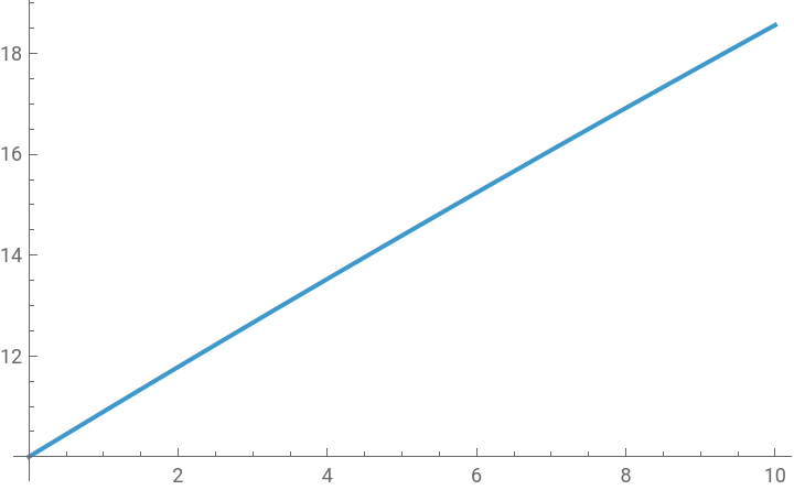
Suppose, for example, b = 1, r = 0.02, g = 0.03, and d0=10, then
In[]:=
Clear[d,d0,r,g,d,b,eqn,sol,t];b=1;r=0.02;g=0.03;d0=10;eqn={d'[t]==(r-g)d[t]+b,d[0]==d0};sol=DSolve[eqn,d[t],t][[1]]
Out[]=
{d[t]100.(-0.9+1.)}
-0.01t
0.01t
In[]:=
Plot[d[t]/.sol,{t,0,10},PlotRange->Automatic]
Out[]=
Alternatively, we can use another Mathematica function, ParametricNDSolve[], to create an interactive solution.
In[]:=
Clear[d,d0,r,g,d,b,eqn,sol,t];b=1;d0=10;eqn={d'[t]==(r-g)d[t]+b,d[0]==d0};sol=ParametricNDSolve[eqn,d,{t,0,10},{r,g}][[1]]
Out[]=
dParametricFunction


In[]:=
Manipulate[Plot[Evaluate[d[r,g][t]/.sol],{t,0,10},PlotStyle{Red,Thick},PlotRange->{0,50}],{{r,0.02},0.01,0.2},{{g,0.03},0.01,0.15},SaveDefinitions->True]
Out[]=


Conclusion
Conclusion
This note demonstrates how we can derive crucial debt to GDP growth rate from the basic macroeconomic accounting identity. The higher growth rate of GDP decreases the debt to GDP ratio over time given the nominal interest rate and the inflation rate. If the real interest rate is greater than the growth rate of GDP, the government’s existing stock of debt to GDP ratio continues to rise exponentially.
With this core dynamic relationship in mind, one can easily integrate this debt stock growth model with many macroeconomic models including Keynes’s AD model and Hicks’s ISLM model. As long as the macroeconomic model introduces the government debt stock and deficit spending, and as long as we have equations for nominal and real interest rate variables, we can tie them together to show the similar dynamic adjustment pattern.
Reference
Reference
Duncan K. Foley, Understanding Capital - Marx’s Economic Theory. Cambridge: Harvard University Press, 1986.
John M. Keynes, The General Theory of Employment, Money and Interest. New York: Prometheus Books, 1997 [1936].
Landall R. Wray, Understanding Modern Money - The Key to Full Employment and Price Stability. Cheltenham, UK and Northampton, MA, USA: Edward Elgar Publisher, 1998.
Srinivas Raghavendra and Petri T. Piiroinen, An Introduction to Economic Dynamics - Modelling, Analysis and Simulation, Routledge: 2023, pp.79-90.
CITE THIS NOTEBOOK
CITE THIS NOTEBOOK
Introduction to dynamic economic models: The government's fiscal deficit and debt accumulation
by Hee-Young Shin
Wolfram Community, STAFF PICKS, December 14, 2025
https://community.wolfram.com/groups/-/m/t/3590770
by Hee-Young Shin
Wolfram Community, STAFF PICKS, December 14, 2025
https://community.wolfram.com/groups/-/m/t/3590770