The Wolfram Emerging Leaders Program: High School (WELP:HS) is a remote, semester-long program designed for exceptional graduates from the Wolfram High School Summer Research Program to continue to develop their skills. Students work in a small group over the course of a semester to do either a research-based project or a product development–based project under the guidance of expert mentors. Projects are centered around a topic at the intersection of the group’s interests.
◼
With contributions from Eileen Lee
Generating, modeling, and analyzing plastic polymers and other general repeat-unit formulas via a top-level function past SMILES notation that can provide more functionality for polymer characterization does not currently exist. Here, we present a method to generate and modify plastic polymers using the SMILES string representation, including functionality for both simple and complex branching. These plastic polymers are then used to simulate short-chain polymer degradation over time by implementing both physical (beta scission) and chemical (autoxidation) degradation processes.
Introduction
Introduction
Why Plastic Degradation?
Why Plastic Degradation?
Plastic pollution has become one of the most persistent environmental challenges of the modern era. Plastics are durable, lightweight, and inexpensive, which have made them a common material in our daily items. Unfortunately, those same qualities make them incredibly resistant to natural degradation. As a result, large quantities of plastics accumulate in landfills, rivers, and oceans, where they then break down and infiltrate ecosystems. The consequences range from harm to wildlife to contamination from additives and pollutants. Understanding how plastics break down in natural environments is essential for potentially addressing the global issue, since accurate models of degradation processes help to predict long-term environmental impacts. Modelling provides a way to quantify the rate of degradation and investigate which key variables influence it. Exploring plastic degradation contributes to the broader effort to understand and ultimately reduce the footprint of plastic materials.
Polymers & Plastic
Polymers & Plastic
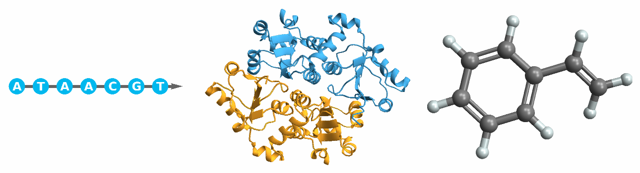
Polymers are typically very large molecules (though not necessarily!) that are made up of repeating subunits of one or more monomers. Essentially, polymers are made up of any number of chained chemical building blocks, and they play major roles for everyday life. While synthetic plastics, like the polystyrene in styrofoam cups might come to mind, other vital molecules, like DNA, proteins, and cellulose, are all polymers.
DNA, insulin proteins, and styrene are all kinds of polymers
In[]:=
GraphicsRowBioSequencePlot[BioSequence["DNA","ATAACGT"]],BioMoleculePlot3D[BioMolecule["3l40"]],MoleculePlot3D
Out[]=
Plastics are a subcategory of polymers; they are a wide range of synthetic materials that can be molded, extruded, or pressed into various shapes and forms (hence the name, because of their “plasticity”). As ubiquitous as they are, their molecular structures are incredibly complex and can be hard to pinpoint to the molecular level. This complexity is largely due in part because of the highly variable processes used to manufacture various plastics, and because of the wide array of properties that plastics can yield based on formulations. There are various measurements of plastics, however, that help to understand a plastic’s structure and properties. Accurately simulating these measurements, even when simulating at the atomic scale, can help apply findings to the larger scale.
Structural Components of Plastics
Structural Components of Plastics
Polyethylene is one of the most commonly used/manufactured plastics globally. However, it also has one of the simplest monomer structures. Despite that, it can be formulated into single use bags, water bottles, and containers. The differences in these materials’ rigidity is the result of multiple differing factors.
Chain Length/Degree of Polymerization
Chain Length/Degree of Polymerization
Since polymers are made of chains of monomers, the length of each individual chain can vary significantly. The average number of enchained monomers is called the degree of polymerization and is directly correlated with the molecular weight/entanglement of the chain. While polyethylene chain length commonly falls between tens to thousands of repeating units, simulations of specific polymer chains often focus on modeling one large chain with a high degree of polymerization to identify various properties, or have a large number of polymers with a smaller degree of polymerization. In our degradation tests, we test polyethylene at low degrees of polymerization to understand the smaller molecular scale of degradation.
Branching & Crosslinking
Branching & Crosslinking
Depending on the type, plastics typically have some level of branching and crosslinking. The rates of these also affects the properties of the plastic. Low-density polyethylene (LDPE) have frequent branching (~2% of the entire backbone is branched), where the backbone has frequent branches of polyethylene (as well as branches of polyethylene connected to other branches of polyethylene, and so on). High-density polyethylene, is linear with little to no branching, resulting in more rigid materials.
In addition, branches can be considered long-chain branches (60+ carbon atoms) or short chain atoms (~5-10 carbon atoms). Linear low-density polyethylene has no long-chain branches but a number of short-chain branches.
Crosslinking is when multiple polymer chains are connected together, and results in increased durability/strength of the final material.
Semi-Crystalline/Amorphous Structures
Semi-Crystalline/Amorphous Structures
Plastics also uniquely can have both semi-crystalline and amorphous structures within the same polymer. Polymers can form a more rigid semi-crystalline structure with ordered and tightly packed molecular chains (like in high-density polyethylene) as well as amorphous structures that are disordered and entangled regions (like in LDPE).
Polymers in Wolfram
Polymers in Wolfram
Currently, the Wolfram language does not have top-level functionality for repeat-units of general polymers (except for its support with biomolecules) past Simplified Molecular Input Line Entry System (SMILES) strings. Higher-level functions could provide more features and hold subvalues for polymer characterization, like degree of polymerization. While there are many possible approaches for modeling polymers in Wolfram, our work in this project uses the aforementioned SMILES strings to provide a method to create polymer generating functions and modification.
Types of Plastic Degradation Models
Types of Plastic Degradation Models
Plastic degradation in the environment proceeds through multiple interconnected mechanisms, but among the most influential are chemical degradation through autoxidation and physical fragmentation driven by beta scission. Autoxidation involves a sequence of radical-mediated reactions, introducing oxygen-containing functional groups and weakening the polymer backbone of a singular plastic piece. Beta scission represents the actual physical breaking of polymer chains, and it produces smaller fragments that eventually become microplastics.
Although these process are linked, autoxidation is often the precursor for beta scission, they arise from distinct mechanisms and operate on different timescales. While autoxidation is governed by chemical kinetics and a sequence of reactions involving radicals, beta scission is driven by chain cleavage. Investigating them separately allows us to explore the unique variables that affect each pathway and provide a clearer framework for a model, since chemical changes and physical fragmentation produce different measurable outcomes.
Although these process are linked, autoxidation is often the precursor for beta scission, they arise from distinct mechanisms and operate on different timescales. While autoxidation is governed by chemical kinetics and a sequence of reactions involving radicals, beta scission is driven by chain cleavage. Investigating them separately allows us to explore the unique variables that affect each pathway and provide a clearer framework for a model, since chemical changes and physical fragmentation produce different measurable outcomes.
Modeling Polymers
Modeling Polymers
Simple Chains
Simple Chains
For our demonstrations, polyethylene (PE) is used as the model plastic because of its simple monomer characterization as purely an alkene (a hydrocarbon with carbon-carbon double bonds) and its prominence as one of the most manufactured plastics. Polyethylene has been estimated to account for around 30% of global plastic waste (Qiao et al., 2026).
Any chemical within Wolfram can be depicted using its Simplified Molecular Input Line Entry System (SMILES) structure information.
Depict an ethylene molecule through the SmilesPlot function:
In[]:=
ResourceFunction["SmilesPlot"]["C=C"]
Out[]=
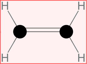
During the polymerization process, ethylene replaces its double bond with a single bond to bind with other carbons, becoming a carbon-carbon single bond. When polymers are being modeled, this different polymer structure needs to be accounted for. A segment of polyethylene can be represented through SMILES as well.
Plot a tetramer of polyethylene:
In[]:=
MoleculePlot3D["CCCCCCCC"]
Out[]=

Formation of polyethylene polymer chains is done quite easily with SMILES strings, with it simply being a joining of carbon atoms.
Use the chained monomer to form any chain-length of polyethylene
In[]:=
makeNChainPolymer[n_,backboneMonomer_]:=StringJoin[backboneMonomer,Table[backboneMonomer,n-1]]
In[]:=
MoleculePlot3D[makeNChainPolymer[20,"CC"]]
Out[]=

More Complex Chaining
More Complex Chaining
A similar process can be applied to more complex molecules, as long as a chemical structure for the chained monomer is defined. In many polymerization reactions, there is some loss of atoms, such as the dehydration synthesis/condensation reaction of polylactic acid, a biodegradable polymer commonly used in 3D printing.
Visualize the monomer structure of lactic acid:
In[]:=
MoleculePlot3D["SMILES"]
Out[]=

To form polylactic acid, the monomer’s oxygen end (bonded to the carbon with a double-bonded oxygen) would bond to another monomer’s central carbon (bound to two other carbons), replacing the originally bound oxygen to form an excess water molecule. Note that in order for the same function used for polyethylene to function, the last atom in the SMILES string must be the atom that bonds to the beginning of the SMILES string. In this case, the last atom, the single oxygen molecule, binds to the central carbon atom, which has been placed first. This format is able to be obtained through repeat-unit formulas of most polymers. For example, the repeat-unit formula for polylactic acid is:
)HC(=O)O–
This formula can then be converted into a SMILES string, and special care must be taken to make sure that the conversion accurately represents the repeated unit.
[–C(
CH
3
]
n
This formula can then be converted into a SMILES string, and special care must be taken to make sure that the conversion accurately represents the repeated unit.
Repeat-unit formula of polylactic acid converted into SMILES:
In[]:=
MoleculePlot3D["C(C)C(=O)O"]
Out[]=

Apply the same function to form polylactic acid chains.
In[]:=
MoleculePlot3D[makeNChainPolymer[3,"C(C)C(=O)O"]]
Out[]=

To visualize each monomer unit, use a MoleculePattern to highlight each corresponding unit inside the molecule plot.
In[]:=
MoleculePlot3D[makeNChainPolymer[3,"C(C)C(=O)O"],MoleculePattern["C(C)C(=O)O"]]
Out[]=

Simple Branching
Simple Branching
To better simulate realistic plastics, branching can also be achieved when creating polymer chains. There are two common types of branching: simple and complex branches, where simple branching is from the chain backbone, such as in linear low-density polyethylene (LLDPE)and complex branching includes branching off simple branches, seen in low-density polyethylene (LDPE). Branches can also be considered long-branched (in LDPE) and short-branched (in LLDPE).
Branches can be added through modifying the SMILES string of the polymer, adding a branch wrapped in parentheses.
A tetramer with a 2-unit long branch
In order to randomize the branching within a chain, string functions can be used to randomly select a valid backbone atom for a branch to be added.
First, the starting polymer chain is converted into a list so an index can be randomly selected:
Any carbon backbone atom is valid for a branch to be added:
Randomly select index to add a branch to, verify that there is not a branch already bound to the chosen atom:
Combine functions to add any given number of branches to a backbone, repeatedly:
Insert three randomly placed branches into the polymer:
While this process may generate polymers that appear to have complex branching, only simple branching is possible with this function. The function allows any valid atoms in the backbone polymer to have branches, but branches are not allowed to form extra branches.
Complex Branching
Complex Branching
To create complex branching, the starting polymer list needs to be re-evaluated every time a branch is added, and allow for branches to be valid locations for branching. Using the simple branching as a base, startingPolymerList is instead evaluated within the function, and the function checks if its current atom location is valid for a branch (making sure that there are not two branches to one atom). Since the complex branching function re-evaluates the polymer list, the complex branch function converts its list into the SMILES string final output, instead of being done in the multi-branch function.
Modify simply branching function to consider branched items by re-evaluating startingPolymerList:
Only Nest is necessary to iterate since the conversion is done within the prior function:
This function does not guarantee complex branching, but is a randomized process where complex branching is allowed, corresponding to random polymerization processes.
Chemical Degradation by Autoxidation
Chemical Degradation by Autoxidation
Location and Key Features
Location and Key Features
Chemical degradation occurs commonly in many of our known environments, as its driven by regular environmental conditions. Oxygen exposure is the key factor, as the name also suggests, but it helps to form peroxy radicals. Sunlight and heat are also important for the rapid propagation of radicals on the carbon backbone. This kind of degradation can occur in any kind of environment sun-exposed, so ocean surfaces, beaches, landfills to name a few. These settings are especially relevant because they are widespread and heavily impacted by human activity. Ocean surfaces and beaches consistently experience high temperatures, strong sunlight, and potential mechanical wear from water or sand. While landfills are a bit less obvious since the plastic is less sun-exposed, plastics can be left partially uncovered which drives slow but persistent degradation. This kind of degradation is not rare or isolated, but it continuously happening across the planet.
Mechanism & Code
Mechanism & Code
Autoxidation proceeds through a well-defined chain mechanism in a series of events, where organic molecules can react with oxygen to form organic hydroperoxides. Those break down further into radicals and products. When looking at plastic degradation, we can see how these changes over time weaken a singular piece of plastic.
The beginning of the process is initiation, where radicals (unpaired electrons) are formed. These radicals can form on the carbon chain through heat, light, catalysts, and other peroxide decomposition.
Initiation: we assign the polymer a radical to begin with:
Here is an example with a 14-carbon chain. We must keep track that the radical is on the 4th carbon, as this will one of our arguments when doing future steps.
The next step is to convert the carbon radical into a peroxyl radical. Since oxygen has two unpaired electrons in its ground state, it reacts extremely fast with carbon radicals.
We add oxygens to create a ROO* group on the polymer:
On our initiated chain from above:
OxygenQ helps to keep track of the peroxy oxygens that we created above:
The polymer then undergoes propagation, which is the formation of an ROOH group. The ROO* that was formed above abstracts a hydrogen from the environment or a nearby RH group, and forms ROOH. Since a hydrogen was abstracted, we’re left with another radical, and this continues the chain.
Propagation creates hydroperoxides ROOH and new polymer radicals to continue the chain reaction:
Propagation on the 14-carbon chain, letting the new radical be on the 7th carbon:
Hydroperoxides are unstable and break down into new radicals. The pathway coded here is homolytic cleavage, in which an ROOH group decomposes into RO* and HO*. Another potential reaction here is metal-catalyzed decomposition. Reducing agents such as iron often accelerate this process.
ROOH decomposes, so our ROOH becomes RO* + *OH:
ROOH decomposition:
The sequence of steps above, propagation and ROOH decomposition can continue to occur as long as a radical is present. Due to the constant regeneration of new radicals, oxidation can accelerate once it starts. There are a couple potential stopping points depending on the availability of radicals. The first is recombination, in which two radicals combine to form a stable product. Another pathway is disproportionation, in which two radicals can gives us two non-radical products involving hydrogen transfer. The difference is that disproportionation often produces unsaturated products.
Recombination takes two radicals and they become a single bond. Disproportionation takes two radicals and clears them both, creating a C=C instead:
From this, we can track molar mass over time for autoxidation to see how much our polymer has been chemically affected.
The steps of autoxidation can also be run on a longer chain polymer, done below. We first choose a random carbon for the radical.
Since we are left with more radicals on the carbon chain, the autoxidation process can continue repetitively.
Physical Fragmentation by Beta Scission
Physical Fragmentation by Beta Scission
Location
Location
Physical fragmentation often dominates where there is physical abrasion, potentially caused by waves, wind, animals, and human activity. Typically, fragmentation can occur on shorelines, rivers, ocean surf zones, fields, and urban environments, all places commonly littered with plastics. Eventually in these environments, these physical factors create microplastics, which introduces a whole new set of dangerous medical issues once they enter the body.
Mechanism
Mechanism
Beta scission occurs when a free radical on a polymer chain undergoes cleavage at the bond located at the beta carbon relative to the radical site. The radical carbon’s neighbor is the alpha carbon, whose other neighbor is what we call the beta carbon. The intention and driving force behind the process is to form a more stable radical. Through this repetitive process, the radical is moved around carbons. In environmental degradation, beta scission is the step that reduces molecular weight, creates shorter polymer fragments, and produces volatile products. This makes beta scission the main contributor for formation of microplastics and nanoplastics. Autoxidation often introduces these radicals on the polymer chain, and so the two processes are sequential.
Simulation in code
Simulation in code
Beta scission is when the bond between an alpha and beta carbon is broken. We create a few helper functions in order to identify the carbons we can work with:
Creating neighbor functions that return the indices of the neighbors of a certain element:
As with autoxidation, we first need a radical to initiate the process. However, this must be a backbone carbon. We test for a backbone carbon by seeing if a given carbon has more than two carbon neighbors, and thus is not on the end of a chain.
The backboneCarbonQ checks to see if the carbon we’re working with is a backbone carbon:
Selecting our backbone carbons:
To kick off the process we need to have a radical, so we assign one at random from the backbone carbons:
A singular beta scission step first checks to see that we have a radical carbon so that we can proceed. Once a radical site is confirmed, the function identifies the alpha carbons, which are simply the carbons directly bonded to the radical carbon. They are the immediate neighbors of the radical center. From the list of alpha carbons, we then identify the corresponding beta carbons. These are the atoms bonded to the alpha carbons but not the radical itself. After collecting all valid alpha/beta pairs, the function evaluates which pairs represent a chemically reasonable site for bond cleavage. It then breaks the bond and updates the chemical structure accordingly. This mirrors the chemical logic of fragmentation and ensures beta scission can only be performed when allowed.
A singular beta scission step:
Now after beta scission we will get a list of “fragments” which we want to continue to do beta scission on.
To clean things up, we run a labelled simulation that tells us the fragments at each step and the largest fragment size.
Example:
We can now track largest fragment size versus step based on what we just ran.
We can run this process many times to determine what size fragments resulting from the breakdown of a polymer is most likely.
Grab results from running the beta scission function 1000 times:
Retrieve carbon length data from the test results:
Organize the data, tallying the corresponding number of cases to the fragment size:
Represent our data on a bar chart:
Estimating Time of Degradation
Estimating Time of Degradation
Kinetics
Kinetics
In any degradation pathway, the rate at which reactions occur determines how quickly a polymer transitions from an intact material to a fragmented one. Kinetics provide the framework for describing these rates. This is through a rate constant, denoted k, which captures how fast a given step happens under specific conditions. A rate constant allows one to express a step in a reaction using an equation dependent on the factors in the reaction.
Rate Constants for Beta Scission
Rate Constants for Beta Scission
Beta scission is treated as a first-order process. Here we can assume an effective rate constant k=1.0 for the simulation. Instead of tracking how the rate constant might differ from step-to-step, we rather let there be a randomly determined time gap between the steps. This allows us to take into account how chemical reactions are not always consistent, and often neither are the environmental factors.
Running a random history of the beta scission against time with rate constant k=1.0
A sample largest fragment size graph that could result from the above calculation:
Other Factors for Degradation
Other Factors for Degradation
There are several different changing factors in the environment, such as varying levels of UV radiation, sunlight exposure, temperature, oxygen availability to name a few. The behavior of each of these can accelerate or modify degradation. UV light is one of the strongest drivers of polymer degradation, initiating photo-oxidation and generating radicals which start autoxidation. It dramatically increases degradation time, but varies due to latitude, season, clouds, and exposure time. Sunlight can compound on this, often amplifying existing chemistry while not making much difference on its own. Depending on the composition of the plastic, water and microbes also play a huge role. However, in a plastic like polyethylene, the C-C backbone is not affected much by these factors. Similarly, changing pH of the environment does not change the polymer’s processes.
Mathematically Modeling the Effects of Pressure and Temperature on Rate
Mathematically Modeling the Effects of Pressure and Temperature on Rate
There are some factors that we know can have incredibly significant effects, and whose effects can be modelled mathematically. Temperature is one of the most influential environmental variables, with even small increases dramatically accelerating radical formation and chain scission. While pressure does not get as much attention, it affects both oxygen availability and mechanical stress. The amount of oxygen that dissolves or diffuses through the polymer controls the rate of oxidation and radical propagation. In order to see the effects of these environmental parameters on the rate of reaction, we can use existing mathematical models to modify the rate constant.
Retrieving gas constant and Arrhenius equation:
Putting some reasonable values to start with, and being able to output a value for k:
We can do a similar thing for pressure with the following equation:
A high altitude corresponds to a lower pressure:
By running values into these equations, several patterns emerge and we get key results for the rate of plastic degradation. Firstly, increasing the temperature will give us higher rate constants, indicating degradation occurs faster in warmer environments. A lower pressure, so a higher altitude, gives us a lower rate constant. This signifies that places at a higher elevation likely will have degradation occur at a slower rate. A very fast rate of degradation can be dangerous as it results in the rapid formation of microplastics. Thus, environments under intense heat or UV exposure might have more significant health risks due to microplastics in comparison to communities in high-elevation environments.
Conclusion & Discussion
Conclusion & Discussion
Polymer Generation
Polymer Generation
Our polymer generating functions are able to generate any length of polymer because of its string representation and can be modified to represent most kinds of plastic polymers. However, these functions do not represent the actual polymerization reaction of the polymer and instead is a “shortcut” to represent what the polymer chemical representation would be. While this method prevents the created polymer generation functions from being applicable in analyzing and testing polymer generation, it does make polymer generation, especially when hundreds to thousands of monomer units are needed, much faster and simpler. These functions also require knowledge of the polymer’s repeat-unit formula, and a repeat-unit formula may need to be created and verified that the SMILES string accurately represents the monomer repeat unit.
Function Limitations and Assumptions
Function Limitations and Assumptions
For simplicity, we assume single pathways such as autoxidation and beta scission. In reality, radicals might undergo many different processes and rearrangements. In the presence of metals and other environmental factors, molecules often follow alternate mechanisms. Additionally, probability of bond breakage is determined by factors such as bond dissociation energies, activation barriers, and stability of the reduction molecules. Here, we assume bonds have equal probabilities given they are a valid alpha-beta pair. We let our rate constant equal 1.0 for each step, but rate can vary step-to-step dependent on radical availability, concentration, and specific geometry of the molecule. While real radical chemistry is complex and relies on thermodynamics, resonance, and steric effects, we let molecular connectivity decide oxidation and fragmentation.
Future Applications
Future Applications
Further modification of our functions can be used to represent more complex plastic systems, such as networks and copolymers. The usage of SMILES strings was convenient for our purposes with polyethylene, but our approach may not be universally applicable for more complex monomers/representations. Modification of the branching approach is needed for crosslinked/network representations, and copolymers can be applied by modifying our chain creation method. However, using SMILES strings does not completely simplify polymer generation -- there must be careful representation of monomer repeat units to ensure that concatenation can accurately form the polymer. Using SMILES strings to represent polymers requires close attention to formulas to ensure accurate creation and will require more work to generalize to any given plastic representation. But, using SMILES representation does have enough adaptability in its syntax to represent polymers accurately without the need for the characterization of the polymerization reaction.
Acknowledgements
Acknowledgements
We would like to express our deepest appreciation for the extensive guidance, review, and experience/knowledge provided by Dr. Jason Sonnenberg, who mentored this WELP project. We would also like to thank Eileen Lee for her contributions for project direction and preliminary research. In addition, Rory Foulger and Eryn Gillam’s thorough feedback for our project in all of its phases greatly helped us throughout our process.
References
References
In order of appearance:
1
.Rudin, A., & Choi, P. (2013). Introductory Concepts and Definitions. In The Elements of Polymer Science & Engineering (pp. 1–62). Elsevier. https://doi.org/10.1016/B978-0-12-382178-2.00001-8
2
.Qiao, J., Wu, L., Ma, X., Li, A., Tian, Y., Lin, H., Guo, D., & Li, X. (2026). Advances in polyethylene biodegradation and bioconversion: Microbial, enzymatic, and biotechnological insights. Engineering Microbiology, 6(1), 100255. https://doi.org/10.1016/j.engmic.2025.100255
3
.Chamas, A., Moon, H., Zheng, J., Qiu, Y., Tabassum, T., Jang, J. H., Abu-Omar, M., Scott, S. L., & Suh, S. (2020). Degradation Rates of Plastics in the Environment. ACS Sustainable Chemistry & Engineering, 8(9), 3494–3511. https://doi.org/10.1021/acssuschemeng.9b06635
4
.Baldera-Moreno, Y., Pino, V., Farres, A., Banerjee, A., Gordillo, F., & Andler, R. (2022). Biotechnological Aspects and Mathematical Modeling of the Biodegradation of Plastics under Controlled Conditions. Polymers, 14(3), 375. https://doi.org/10.3390/polym14030375
CITE THIS NOTEBOOK
CITE THIS NOTEBOOK
Simulating plastic polymer degradation
by Advika Asthana, Max Wang, and Eileen Lee
Wolfram Community, STAFF PICKS, February 11, 2026
https://community.wolfram.com/groups/-/m/t/3638297
by Advika Asthana, Max Wang, and Eileen Lee
Wolfram Community, STAFF PICKS, February 11, 2026
https://community.wolfram.com/groups/-/m/t/3638297