Here we define a reflection operator, and a function to find line-cylinder intersections:
In[]:=
SetDirectory[NotebookDirectory[]];δ=10^4$MachineEpsilon;Clear[Sgn,Reflect,RayCylinderIntersection](*worksslightlydifferentfromthebuilt-inSign:Sign[0]=0versusSgn[0]=1*)Sgn[x_]:=If[x<0,-1,1]Reflect[ii_,in_]:=Normalize[ii-2(ii.in)in]RayCylinderIntersection[{pt1:{x1_,y1_},k:{u_,v_}},r_]:=Module{dr,Δ,d,solx1,soly1,solx2,soly2,τ1,τ2},dr=+;d=vx1-uy1;Δ=-;WhichΔ<0,False,Δ0.,solx1=dv();soly1=-du();IfN[u]=!=0.,τ1=,τ1=;If[τ1>0,{τ1,τ1k+pt1},False],True,solx1=dv+Sgn[v]u;IfN[u]=!=0.,τ1=;τ2=;,τ1=;τ2=;;τ1=Min[Select[{τ1,τ2},#>δ&]];If[τ1=!=∞,{τ1,τ1k+pt1},False]
2
u
2
v
2
r
2
dr
2
d
2
dr
2
dr
solx1-x1
u
soly1-y1
v
Δ
;soly1=-du+Abs[v]Δ
;solx2=dv-Sgn[v]uΔ
;soly2=-du-Abs[v]Δ
;{solx1,soly1,solx2,soly2}/=2
dr
solx1-x1
u
solx2-x1
u
soly1-y1
v
soly2-y1
v
This will compute the nearest intersection:
ClearAll[DoStep]DoStep[path_List,pts_List,r_]:=Module[{last=Last[path],p,v,newp,ord,out},{p,v}={last["p"],last["v"]};newp=(p-#)&/@pts;ord=Ordering[Norm/@N[newp]];Do[out=RayCylinderIntersection[{newp[[o]],v},r];If[out=!=False,out={out[[2]],newp[[o]]};Break[]];,{o,ord}];If[out=!=False,Append[path,<|"p"->out[[1]]-out[[2]]+p,"v"->Reflect[Normalize@v,Normalize@out[[1]]]|>],path]](*makesomecylinders,anddo50bounceseach*)r=2/5;size=12;pts=Catenate@Table[i{1,0}+j{0,1},{i,-size-1/2,size+1/2},{j,-size-1/2,size+1/2}];(*pts=Table
i
AngleVector[iGoldenAngle],{i,1,1000};*)Dynamic[N@θ]allpaths=Table[path={<|"p"->{0`150,0`150},"v"->AngleVector[N[(21+θ/1000000000000)Degree,150]]|>};path=Nest[DoStep[#,pts,r]&,path,50];path,{θ,-5,5,1/20}];colors=ColorData["Rainbow"]/@Subdivide[Length[allpaths]-1];Graphics[{Thickness[0.002],Riffle[colors,Line/@allpaths[[All,All,"p"]]],Black,Disk[#,r]&/@pts}]Out[]=
θ
Out[]=
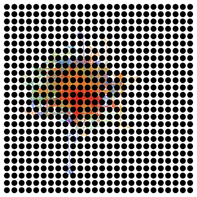
What is the spread of the endpoints of the lines at some distance d, to determine the plot range:
In[]:=
ClearAll[LineUptoLength]LineUptoLength[pts_List,d_]:=Module[{sizes,accsize,len,new,rest},If[d<=0,{},sizes=Norm/@Differences[pts];accsize=Prepend[Accumulate[sizes],0];If[d>=Last[accsize],pts,len=LengthWhile[accsize,LessEqualThan[d]];rest=d-accsize[[len]];new=pts[[len]]+restNormalize[pts[[len+1]]-pts[[len]]];Append[pts[[;;len]],new]]]]Show[{ListPlot[Table[{d,2Norm[StandardDeviation[Identity[Last[LineUptoLength[#[[All,"p"]],d]]&/@allpaths]]]},{d,0.1,30,1}],PlotRange->{0,10}],Plot[1.2+6LogisticSigmoid[d-7],{d,0,30}]}]
Make a nice movie:
Render images and export:
CITE THIS NOTEBOOK
CITE THIS NOTEBOOK
Bouncing rays in a grid of cylinders: 20-trillionth degree difference
by Sander Huisman
Wolfram Community, STAFF PICKS, September 20, 2021
https://community.wolfram.com/groups/-/m/t/2369872
by Sander Huisman
Wolfram Community, STAFF PICKS, September 20, 2021
https://community.wolfram.com/groups/-/m/t/2369872