In[]:=
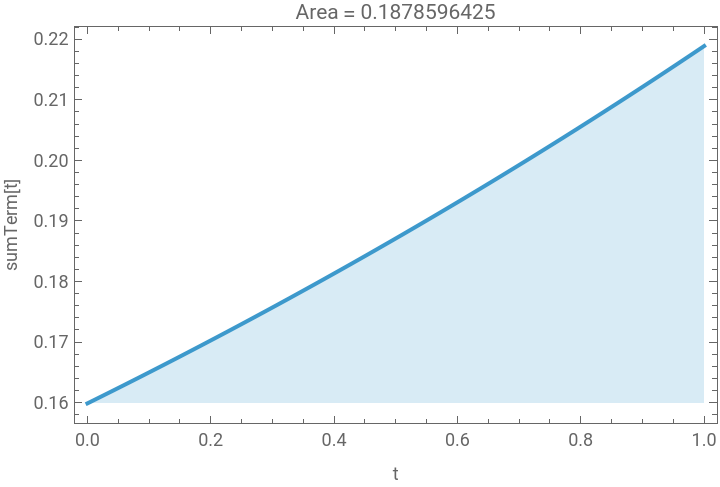
With[ {area=NIntegrate[sumTerm[t],{t,0,1}]}, Plot[ sumTerm[t], {t,0,1}, Filling->Axis, Frame->True, FrameLabel->{"t","sumTerm[t]"}, PlotLabel->Row[{"Area = ",NumberForm[area,10]}] ] ]

n
(-1)
0.0000204286
n
n
Out[]=
In[]:=
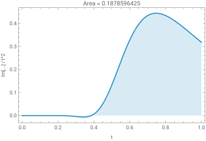
expr=Im[((1-I(1-t)/t)^(1/(1-I(1-t)/t))Csch[Pi(-1+t)/t])/t^2];area=NIntegrate[expr,{t,0,1}];Plot[expr,{t,0,1},Filling->Axis,PlotRange->All,PlotPoints->100,MaxRecursion->6,Frame->True,FrameLabel->{"t","Im[...] / t^2"},PlotLabel->Row[{"Area = ",NumberForm[area,10]}]]
Out[]=
In[]:=
CMRB=-1+;
∞
∑
n=1
n
(-1)
1
n
n
In[]:=
∞
∫
1
Log[n]
n
∫
0
u
Out[]=
0.18786
In[]:=
NIntegrate[-I((1+It)^(1/(1+It))-1)/Sinh[Pit],{t,0,1,Infinity}]
Out[]=
0.18786-0.101409
In[]:=
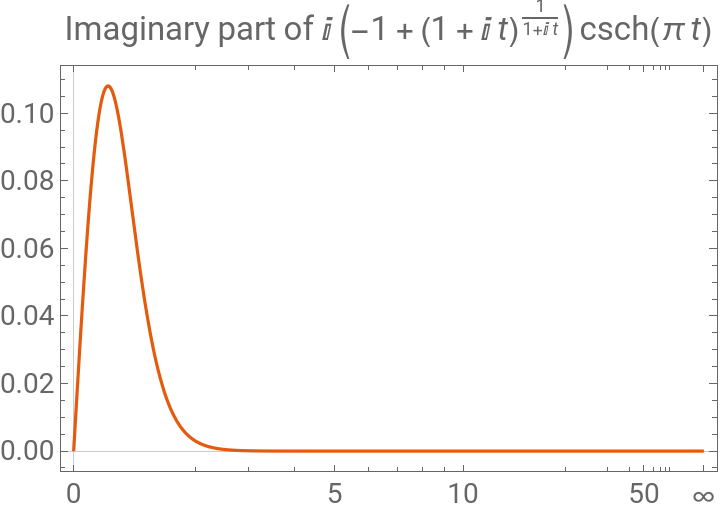
Plot[Im[I((1+It)^(1/(1+It))-1)/Sinh[Pit]],{t,0,Infinity},PlotRange->Full,AxesLabel->{"t","value"},PlotLabel->Row[{"Imaginary part of ",TraditionalForm[I((1+It)^(1/(1+It))-1)/Sinh[Pit]]}],LabelStyle->Directive[14],PlotTheme->"Scientific"]
Out[]=
}
In[]:=
f[n_]:=;2CMRB-u//N
2
Log[n]
∞
∑
n=1
f'[n]
∫
0
u/2-πn
In[]:=
f[n_]:=;u
2
Log[n]
∞
∑
n=1
f'[n]
∫
0
u/2-πn
Out[]=
∞
∑
n=1
-nπ
1
n
n
In[]:=
f[n_]:=;1/2u//N
2
Log[n]
∞
∑
n=1
f'[n]
∫
0
u/2-πn
Out[]=
0.18786
In[]:=
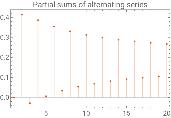
DiscretePlot[Sum[(-1)^n(n^(1/n)-1),{n,1,m}],{m,1,20},AxesLabel->{"m","partial sum"},PlotLabel->"Partial sums of alternating series",LabelStyle->Directive[14],PlotTheme->"Scientific"]
Out[]=
In[]:=
CMRB-log(n)u
∞
∑
n=1
n
(-1)
-1
n
1
∫
0
u/n
n
Out[]=
0
In[]:=
DiscretePlot[(-1)^n(n-1)/(n^2Log[n]^2),{n,2,20},AxesLabel->{"n","summand"},PlotLabel->"Summand of the series",LabelStyle->Directive[14],PlotTheme->"Scientific"]