Fujitsu is advancing the development of quantum computers, so I’ve been seeing more articles about quantum computing within the company. Although I am not involved in the development, I became interested and began studying quantum computers.
Amidst many complex explanations using circuit diagrams, I found a geometric explanation of Grover’s algorithm—one of the fundamental algorithms—particularly helpful for deepening my understanding. The video(Japanese) visually illustrating its behavior was especially insightful.
Based on this knowledge, I implemented a similar algorithm using the Wolfram Language.
Grover’s algorithm
Grover’s algorithm
Grover’s algorithm is a quantum algorithm that, for an unsorted database with N entries, can find a specific entry in roughly O() times, compared to the classical algorithm which takes O(N) times.
N
Classical Search:
Imagine a phone book where the names are not alphabetized. If you’re looking for a specific person, you have to go through each entry, one by one, until you find them. On average, you’d check about half the entries N/2. In the worst case, you’d check all N entries.
Imagine a phone book where the names are not alphabetized. If you’re looking for a specific person, you have to go through each entry, one by one, until you find them. On average, you’d check about half the entries N/2. In the worst case, you’d check all N entries.
Quantum Superposition:
Grover’s algorithm starts by putting all possible entries into a quantum superposition. This means the algorithm “looks at” all entries simultaneously.
Grover’s algorithm starts by putting all possible entries into a quantum superposition. This means the algorithm “looks at” all entries simultaneously.
Amplitude Amplification:
The core of the algorithm is a technique called “amplitude amplification.” It works by iteratively increasing the probability amplitude of the desired entry while decreasing the amplitudes of the incorrect entries. Think of it like shining a spotlight on the correct answer, making it brighter with each step.
The core of the algorithm is a technique called “amplitude amplification.” It works by iteratively increasing the probability amplitude of the desired entry while decreasing the amplitudes of the incorrect entries. Think of it like shining a spotlight on the correct answer, making it brighter with each step.
Measurement: After a certain number of iterations (which is proportional to ), when you measure the quantum state, you have a very high probability of finding the desired entry.
π
4
N
A simple example
A simple example
First, install and load the QuantumFramework paclet
In[]:=
PacletInstall["Wolfram/QuantumFramework"]Needs["Wolfram`QuantumFramework`"];
Out[]=
PacletObject

If N is set to 32=(5 qubits), a classical algorithm can search it in an average of 16 times. However, Grover’s algorithm can search it in 4 times.
5
2
n=;
5
2
Initial state(superposition) for the circuit :
In[]:=
ψ0=QuantumState[{"UniformSuperposition",5}];ψ0["Formula"]
Out[]=
1
4
2
1
4
2
1
4
2
1
4
2
1
4
2
1
4
2
1
4
2
1
4
2
1
4
2
1
4
2
1
4
2
1
4
2
1
4
2
1
4
2
1
4
2
1
4
2
1
4
2
1
4
2
1
4
2
1
4
2
1
4
2
1
4
2
1
4
2
1
4
2
1
4
2
1
4
2
1
4
2
1
4
2
1
4
2
1
4
2
1
4
2
1
4
2
In the initial state, the probability of observing any of the 32 patterns is identical at 1/32.
In[]:=
ψ0["ProbabilityList"]
Out[]=
,,,,,,,,,,,,,,,,,,,,,,,,,,,,,,,
1
32
1
32
1
32
1
32
1
32
1
32
1
32
1
32
1
32
1
32
1
32
1
32
1
32
1
32
1
32
1
32
1
32
1
32
1
32
1
32
1
32
1
32
1
32
1
32
1
32
1
32
1
32
1
32
1
32
1
32
1
32
1
32
Define a Boolean function with only one solution :
In[]:=
bf=And@@(Symbol["q"<>ToString@#]&/@Range[5])
Out[]=
q1&&q2&&q3&&q4&&q5
Generate the corresponding Grover circuit using a phase oracle :
In[]:=
g=QuantumCircuitOperator[{"GroverPhase",bf}];g["Diagram"]
Out[]=
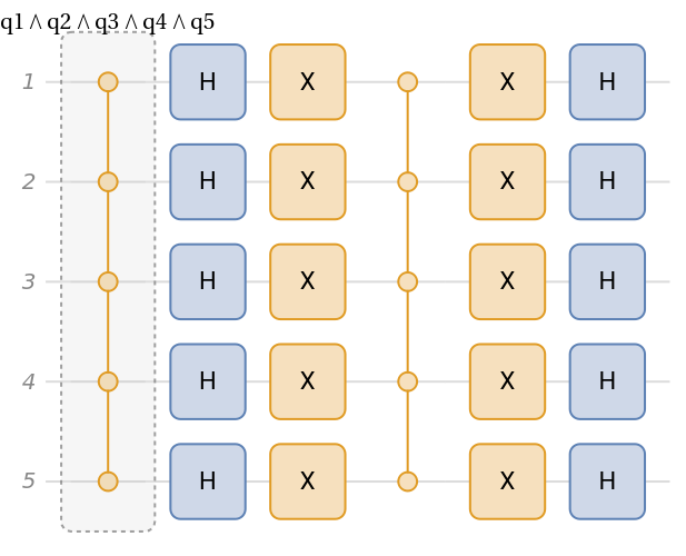
Apply the Grover operator 4 times :
In[]:=
steps=NestList[g,ψ0,4];
The last state :
In[]:=
steps[[-1]]["Formula"]
Out[]=
-|00000〉-|00001〉-|00010〉-|00011〉-|00100〉-|00101〉-|00110〉-|00111〉-|01000〉-|01001〉-|01010〉-|01011〉-|01100〉-|01101〉-|01110〉-|01111〉-|10000〉-|10001〉-|10010〉-|10011〉-|10100〉-|10101〉-|10110〉-|10111〉-|11000〉-|11001〉-|11010〉-|11011〉-|11100〉-|11101〉-|11110〉+|11111〉
119
16384
2
119
16384
2
119
16384
2
119
16384
2
119
16384
2
119
16384
2
119
16384
2
119
16384
2
119
16384
2
119
16384
2
119
16384
2
119
16384
2
119
16384
2
119
16384
2
119
16384
2
119
16384
2
119
16384
2
119
16384
2
119
16384
2
119
16384
2
119
16384
2
119
16384
2
119
16384
2
119
16384
2
119
16384
2
119
16384
2
119
16384
2
119
16384
2
119
16384
2
119
16384
2
119
16384
2
23161
16384
2
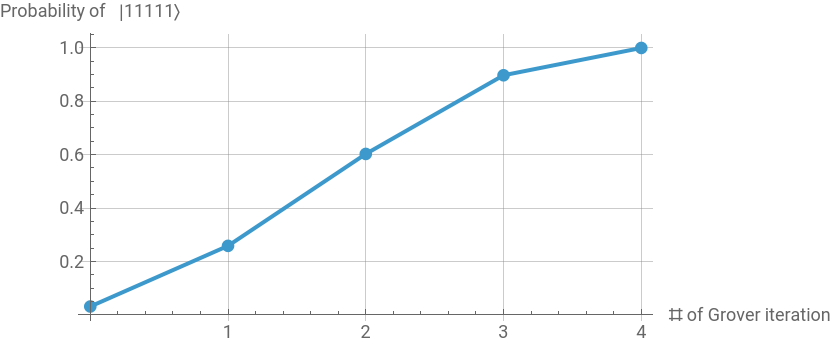
The probability of |11111〉 is = 0.99 :
2
23161
16384
2
Plot the probability of |11111〉 :
In[]:=
prob=#["ProbabilityList"][[-1]]&/@steps;ListLinePlotTranspose[{Range[0,4],prob}],
Out[]=
Geometric interpretation
Geometric interpretation
Since looking at the circuit diagram doesn’t help, explain it using a geometry :
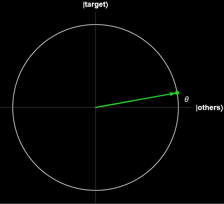
1 State Space:
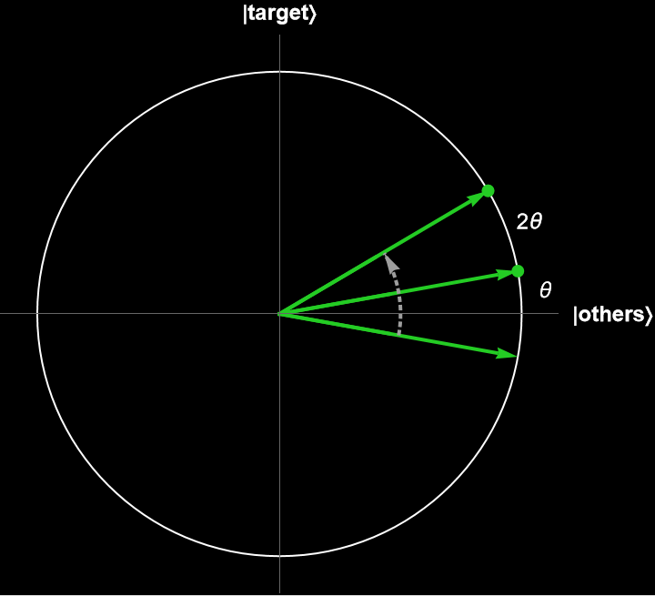
Imagine a 2D plane. One axis represents the amplitude of the “target state” (the state we want to find), and the other axis represents the amplitude of the “superposition of all non-target states.” Our initial uniform superposition state can be represented as a vector in this plane. This vector is initially closer to the non-target states axis.
Imagine a 2D plane. One axis represents the amplitude of the “target state” (the state we want to find), and the other axis represents the amplitude of the “superposition of all non-target states.” Our initial uniform superposition state can be represented as a vector in this plane. This vector is initially closer to the non-target states axis.
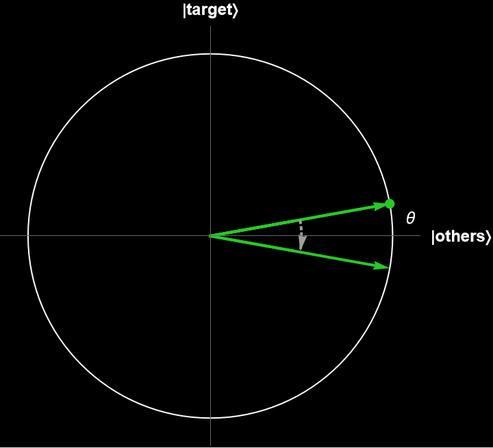
2 Oracle Operation (Reflection 1):
The first step is the “oracle operation.” Geometrically, this acts as a reflection about the axis representing the superposition of non-target states. It effectively “flips” the component of our state vector corresponding to the target state. This means the target state’s amplitude becomes negative, but its magnitude (and thus probability) remains the same. The overall vector is reflected across the “good states are not present” line.
The first step is the “oracle operation.” Geometrically, this acts as a reflection about the axis representing the superposition of non-target states. It effectively “flips” the component of our state vector corresponding to the target state. This means the target state’s amplitude becomes negative, but its magnitude (and thus probability) remains the same. The overall vector is reflected across the “good states are not present” line.
3 Diffusion Operator (Reflection 2):
The second step is the “Grover diffusion operator,” also known as the “inversion about the mean.” Geometrically, this is a reflection about the initial average amplitude vector (our initial uniform superposition state). This operation has the effect of “rotating” our state vector closer to the target state axis.
The second step is the “Grover diffusion operator,” also known as the “inversion about the mean.” Geometrically, this is a reflection about the initial average amplitude vector (our initial uniform superposition state). This operation has the effect of “rotating” our state vector closer to the target state axis.
4 Iteration:
Each pair of these reflections (oracle + diffusion) constitutes one Grover iteration. Each iteration performs a rotation that moves the state vector closer to the target state axis. By repeatedly applying these two reflections, we effectively rotate the state vector towards the desired target state.
Each pair of these reflections (oracle + diffusion) constitutes one Grover iteration. Each iteration performs a rotation that moves the state vector closer to the target state axis. By repeatedly applying these two reflections, we effectively rotate the state vector towards the desired target state.
The number of Grover iteration
The number of Grover iteration
The number of iterations must be carefully chosen to maximize success probability, as over - iteration can reduce the likelihood of finding the correct solution.
Animation and manipulation
Animation and manipulation
Illustrate the behavior of Grover’s algorithm :
Animate 12 qubits :
Manipulate each of the number of qubits and the number of iteration :
CITE THIS NOTEBOOK
CITE THIS NOTEBOOK
Visualizing Grover's algorithm: quantum search for an entry in unsorted database
by Kotaro Okazaki
Wolfram Community, STAFF PICKS, October 23, 2025
https://community.wolfram.com/groups/-/m/t/3564039
by Kotaro Okazaki
Wolfram Community, STAFF PICKS, October 23, 2025
https://community.wolfram.com/groups/-/m/t/3564039