Just as the DNA of an organism can be mutated base-by-base, the rules of a Cellular Automaton (CA) can be mutated bit-by-bit. Leveraging the process of adaptive evolution, this project aims to emulate natural selection on simulated gene pools of CA rules. Out of all the possible attributes to select for, the ability of CA to generate pseudorandom numbers exhibits the most real-world practicality. By first evaluating previous attempts to use CA for cryptographic systems, we will then utilize evolution in order to produce rules that are more random and, as a result, harder to break by methods of cryptanalysis.
Introduction
Introduction
Cellular Automata (CA) are systems that are known for generating emergent, complex behavior from relatively simple rules. Some CA display rather simple behavior over long periods of time and, as a result, can be predicted from initial conditions. For many CA, however, the possibilities after just a couple of iterations become so endless that there is no better way to find a future state than by computing every intermediate state. The basis for any cryptographic system is determinism (the same key needs to always produce the same output) and unpredictability (observing the system should not give any information about future or previous states). Indeed, many CA satisfy these constrains, such as the Rule 30 automaton previously used in Mathematica for generating pseudorandom numbers. This project will present a new method for finding cryptographically-useful CA by using an evolution algorithm to select for desirable traits such as period length and irreversibility. Candidate CA will then be evaluated for practicality and security in the context of an image encryption use-case.
Evaluating Existing Options
Evaluating Existing Options
In 1985, Stephen Wolfram singled out Rule 30 for encryption purposes, introducing the concepts of using the initial state as an encryption key and sampling the center row for random numbers. We will evaluate Rule 30 for cryptographic usefulness, along with other candidates from the well-studied set of 256 possible elementary CA.
Infinite-Grid Rule 30
Infinite-Grid Rule 30
See the output for a single black cell on an infinite grid
In[]:=
ArrayPlot[CellularAutomaton[30, {{1},0}, 100]]
Out[]=
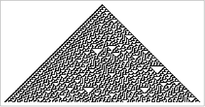
It seems like there’s some regularities on the left side. Let’s take inspiration from the 1985 paper and sample just from the center column.
In[]:=
ArrayPlot[List@CellularAutomaton[30,{{1},0},{100,{{0}}}],Mesh->True]
Out[]=

Could this data be as good as random? Let’s compare the entropy of a larger Rule 30 sample with an equally-sized sample of []
RandomInteger
In[]:=
Entropy[CellularAutomaton[30,{{1},0},{1000,{{0}}}]]//NEntropy[RandomInteger[1,1000]]//N
Out[]=
0.692388
Out[]=
0.693115
Finite-Grid Rule 30
Finite-Grid Rule 30
Rule 30’s center column is seemingly random, but notice that we still have to calculate the entire CA grid to collect our sample. Since the rows become wider as the sample size increases, this method of sampling quickly becomes time-inefficient and impractical for large calculations. Let’s try running Rule 30 on a fixed-width grid to alleviate performance concerns.
16-cell grid with random starting conditions
In[]:=
start=RandomInteger[1,16];ArrayPlot[CellularAutomaton[30,start,100]]
Out[]=

This finite grid isn’t simply a zoomed-in version of the infinite grid -- its behavior is fundamentally different. Firstly, we’ve reduced the amount of possible states from ∞ to , where is the width of the grid. Second, we’ve changed how the automaton behaves with a boundary condition, where rightmost cells consider leftmost cells their neighbor and vice versa. The result of both of these changes is the introduction of periodic behavior. Since there are now a limited number of possible states, and because CAs are deterministic given any initial state, it will take at most rows for the fixed-width Rule 30 to start repeating itself.
In encryption applications, it is crucial that the period of the random number source is significantly larger than the size of the data being encrypted. The rest of this section will attempt to find an elementary rule with a higher period than Rule 30.
n
2
n
n
2
In encryption applications, it is crucial that the period of the random number source is significantly larger than the size of the data being encrypted. The rest of this section will attempt to find an elementary rule with a higher period than Rule 30.
Finding Periods of Finite CA
Finding Periods of Finite CA
For a given rule and starting condition, will create a list of rows up to long, take the last row in the list, search for the first two occurrences, and return the difference between the indices. In order to always find the period, should be set to .
findPeriod[]
iters
iters
n
2
Function to find the period of a CA
In[]:=
findPeriod[rule_, init_, iters_] := Module[{rows, indices},rows = NestList[CellularAutomaton[rule], init, iters];indices = Flatten[Position[rows, Last[rows], 1, 2]];If[Length[indices]===2, Throw[First[Differences[indices]]], -1]]
In[]:=
start={1,1,0,1,0,1,0,0};Catch[findPeriod[30,start,]]
Length[start]
2
Out[]=
40
For this specific starting condition (with ), it seems like Rule 30 will completely repeat itself every 40 iterations. Let’s see if this tracks visually.
n=8
In[]:=
ArrayPlot[CellularAutomaton[30,start,120]]
Out[]=

With a period length of 40 and a simulation of 120 rows, we should see about 3 instances of repeated behavior. We can also see some irregularity at the beginning, hence why uses a reference row from the end of the generated list.
But is this the only possible cycle length for this case? Let’s create a state-transition diagram of every possible 8-bit state and its corresponding Rule 30 iteration.
findPeriod[]
But is this the only possible cycle length for this case? Let’s create a state-transition diagram of every possible 8-bit state and its corresponding Rule 30 iteration.
In[]:=
g=Graph[#->CellularAutomaton[30][#]&/@Tuples[{1,0},8]]
Out[]=
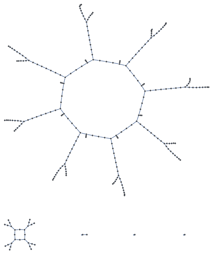
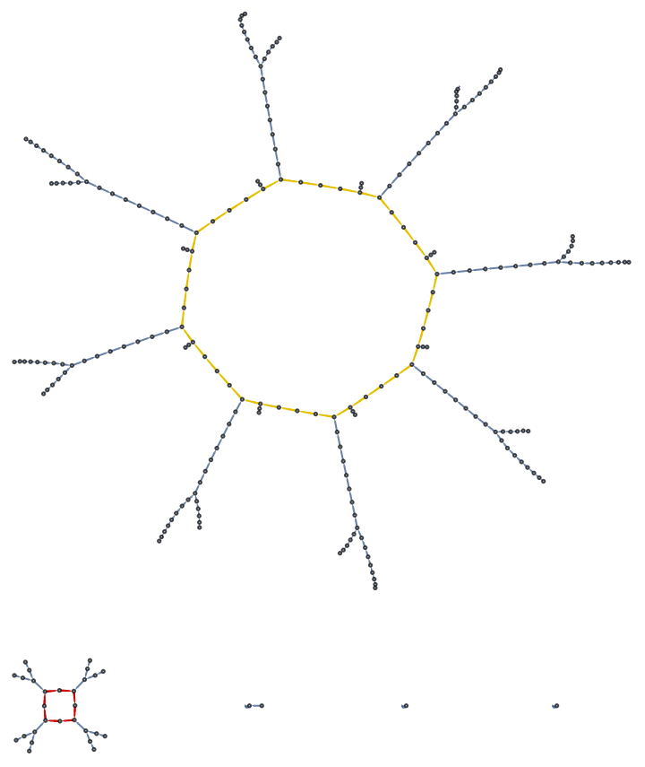
Out of the 256 possible states, it’s not hard to visually locate the cycle of 40 nodes that our initial condition eventually enters. There’s also a number of “transient” paths, but they always lead to a well-defined cycle.
Find all possible cycles in the graph and highlight them
In[]:=
HighlightGraph[g,FindCycle[g,Infinity,All]]
Out[]=
Add a wrapper to increase efficiency of finding a period
Use the wrapper to find maximum period via repeated iteration
Testing findMaxPeriod[] 100 times to see if we ever get a period below the maximum
Finite Cases Besides Rule 30
Finite Cases Besides Rule 30
If we want to find CA which are better than Rule 30 for cryptography, we will generally want to search for rules with higher periods. However, if we simply take a sample at a specific n value, we will quickly run into pitfalls.
Log-scale graph showing the growth of Rule 30’s maximum period
Find the 8 Elementary CA with the largest growth coefficients
Interestingly, Rule 30 is not the highest on our list (even though it is known for random/chaotic behavior). Let’s take Rule 45 from our list and plot it alongside the previous graph.
Just with our simple method of searching the entire set of rules for desirable CA, we’ve found a rule which consistently demonstrates a higher period than Rule 30. Additionally, Rule 45 seems to display the same type of random behavior, which is crucial for encryption candidates.
Rule 45 with infinite and finite grids
However, as we increase the number of possible CA rules (65536 rules for a cell neighborhood of 1.5 and 4294967296 rules for a cell neighborhood of 2), we will need to become much more clever in our search methods.
Creating Evolutionary Fitness Functions
Creating Evolutionary Fitness Functions
If we want to start searching more possible rules for possible candidates, we need to stop wasting time evaluating CA which are useless for encryption. One possible method is to treat each CA like a biological creature, and then follow principles of evolution.
For each candidate, we can apply “mutations” to its rule (analogous to DNA in an organism). For each possible mutation, we will only allow them to “survive” if they become more random/secure. By doing this, we only focus our computations on branches which lead to more desirable rules. Notice how this method assumes that randomness is built up sequentially through small changes. If randomness was instead a property that was completely independent of similarity to other random rules, then we would most likely be skipping branches that contained the most random rules. However, Stephen Wolfram showed the viability for applying evolution to similar properties of CA, such as finite lifespan, in a recent article.
In any case, our evolution algorithm will need a “fitness” function to determine which candidates get to live, and which are cut off from the evolutionary tree. Reversibility and additivity are two properties of cellular automata which our fitness function will filter out due to their undesirability for cryptography.
Reversibility
Reversibility
Some CA have the property of having unique predecessors for every possible state. This is analogous to a function being injective. Let’s create a state-transition diagram to show this property visually.
State-transition diagram for the reversible Rule 15
For each node, there is only one possible path forwards. This means that if we tried to reverse the graph, we would also only have one option for the predecessor state. If we used such a rule for encryption, an attacker could simply “lookup” the previous state until they reached the initial condition (which acts as the encryption key in our implementation). This would effectively break a CA-based encryption algorithm.
If we wanted to test a rule for reversibility, we could simply check for the amount of unique states after one iteration.
If we wanted to test a rule for reversibility, we could simply check for the amount of unique states after one iteration.
Compare Rule 30 input states and output states after one iteration
Boolean function to test for CA reversibility
Find all reversible rules in the elementary CA set and show their state-transition diagrams
Additivity
Additivity
Rule 150 plotted at 10, 100, and 1000 iterations
In addition, additive CA have the property of being reversible horizontally. That is, given a complete column, it is possible to determine a neighboring column. Like regular (vertical) reversibility, this is detrimental for encryption since it allows attackers to gain extra information about the system (perhaps even the key) simply by observing the output states.
Demonstration of horizontal reversibility for Rule 60
Each sublist represents a possible configuration of input cells we can add together. The last sublist, for example, represents adding all three cells together, while the first sublist represents adding none of them together. By applying each one of these additions to all possible input states and then converting the output states to an integer, we can get all rule numbers which are additive.
Since our function already generates an entire list of additive CA, we can make a simple wrapper to check for membership in the additive set.
Finding Symmetries
Finding Symmetries
Wow! That’s a long time. It seems like we’re in need of some optimization.
Discovering the Symmetries
Discovering the Symmetries
Let’s look back at the list of largest periods we made and look for patterns.
It seems like each group of four has a very similar number representing its period growth. Let’s plot each group visually.
The symmetries are easiest to see with the second list. There’s a black-white inversion, a left-right flip, and a combination of both inversion and flipping. This gives us four possible symmetries for each CA rule. This property is very relevant for optimization since all symmetries have the same period as each other (flipping/inverting doesn’t change any of the fundamental patterns of the CA), and thus we never have to recalculate the period of a CA if we already know the period of its symmetry.
Left-Right Symmetry
Left-Right Symmetry
Let’s look at the rule plot for Rule 30.
Of these 8 rules, there are four that would be interpreted differently if we flipped them from left to right. For example, the 111 rule is same when flipped, but the 001 rule becomes 100 when flipped. If we take all of these “flippable” rules, and swap their output bits with the corresponding flipped rule, we will get the left-right symmetry.
Function to get the left-right symmetric version of a CA rule
Let’s check our function for accuracy and visualize how the flipped rule is different from the original.
Notice how all of the symmetric rules stay the same (they essentially swap with themselves) and that all other rules have been swapped with their flipped version. A white-to-white or black-to-black swap doesn’t look like anything, but is still computed.
Black-White Inversion
Black-White Inversion
Function for finding the black-white inversion of a CA rule
Visualize the inverted CA and its rule
Canonicalization
Canonicalization
By combining our functions for both types of symmetries, we can get the fourth symmetry. Let’s create a function that returns all four symmetries at once given a CA rule.
One simple way to canonicalize this data is to take the lowest rule from each set of symmetries. This allows us to make sure we will only have one representative of each symmetric set in our graph, and avoid calculating period length for any other CA in the same set. Let’s create a canonicalization function and see if it generates the same representative for all four Rule 30 symmetries
Get the Rule 30 symmetries and canonicalize them
Through the process of canonicalization, we should be able to reduce our calls to period-finding functions by 4 times!
Generating Evolutionary Trees
Generating Evolutionary Trees
The end result of our evolution algorithm will be a multiway graph that represents all the possible “mutations” that a rule can go through to become better fit for encryption. A child node will be removed if it does not meet or exceed the standard set by its parent node. At the end of the evolution, all “leaf” nodes -- having no children -- will be the fittest representative from their specific evolutionary branch. Since we do not have sufficient time to always generate the entire evolutionary tree, leaf nodes can also be the result of halting our evolutionary early at a specific layer. Still, these leaf nodes will be the best representatives from their incomplete branches, and we will be using them to find the best candidates from our simulations.
Mutations
Mutations
Show all mutations from an elementary CA rule
Hash Table Lookup
Hash Table Lookup
Implementation of a hash table and lookup function
Let’s see how long the first lookup for Rule 30 takes.
Now, on the subsequent access, let’s see how fast we can find the period for Rule 30 and its symmetries.
Integrated Fitness Function
Integrated Fitness Function
After exploring and studying various properties which make CA rules both desirable and undesirable for encryption, it is time to make a singular fitness function which will decide if a mutation lives or dies. Getting rid of these nodes allows us to reach a much further depth without having to waste time backtracking to worse mutations.
Fitness function to get rid of undesirable mutations
3
.Canonicalize every mutation to its representative symmetric form
Constructing Layers and Graphs
Constructing Layers and Graphs
Now that we have functions to generate mutations for a node and evaluate those mutations for fitness, we have everything we need to start building our evolutionary tree. First, let’s create a function to find just the nth layer in the graph -- ignoring nodes on all other layers.
Testing the getNthLayer[] function
The getFullGraph[] function combines all layers of the graph and maintains connections
Testing the getFullGraph[] function evolving from Rule 1
Let’s create a wrapper function to show our connections in graph form.
Testing showGraph[] on our saved connections
Each directed edge shows a possible evolutionary path that a rule can take in order to become more fit for encryption. Note the edges that reach backwards towards a previous layer. These represent “fitness neutral” evolutions, in which two rules have the same period and can freely evolve between each other during the evolution process. Also, notice how some rules have child nodes with rules that differ by much more than one bit. Since our mutation function only operates on one bit at a time, this should be an invalid connection. However, since we canonicalize nodes before storing them in the graph, these connections are simply the result of a single bit flip, and then switching to a different symmetric form.
Larger Simulations
Larger Simulations
Let’s see a graph of the first two layers
If we want to visualize all the connections at once, we can adopt a looser graph structure and get rid of the binary rule representations. In this case, our leaf nodes are still easy to see at the edges, but the other connections become more obscured.
Find the leaf nodes of our graph and print a shortened representation
Since these leaf nodes represent the candidate rules at the end of their respective evolutionary paths, they should represent our most evolved/fittest candidates. Thus, the best leaf node is also the best node from the entire graph.
Find leaf node with highest period
Let’s see how our best rule from five layers of simulation compares to Rule 30
It seems like our new rule has a period that grows significantly faster than Rule 30! Let’s make a plot to show this visually.
That’s only 1% of the entire rule space! Finally, let’s see how this rule looks on a finite and infinite grid.
Image Encryption
Image Encryption
Now that we have used our evolution algorithm to find candidates for encryption, let’s see how they fare in a real-world use-case. Like we did when generating random numbers, we will sample each CA rule from the center row. This stream of random numbers will then be used to XOR every bit in the image stream. As long as our stream of numbers is truly random, it will be impossible to infer the original content of the image. This is because every bit is either flipped (if the key-stream bit is a 1) or remains the same (if the key-stream bit is a 0). If the key-stream is truly random, then it will be impossible to know whether the bit was flipped or not, and thus impossible to know the content of the image. XOR is also a reversible action, so using the same key can both encrypt and decrypt an image (symmetric algorithm). Notice that this method of encryption relies on the four following assumptions:
1
.The period length of the key must be larger than the length of the data. If this is not the case, patterns may be seen in the ciphertext (encrypted data), allowing an attacker to find the plaintext (original message) through methods of cryptanalysis. With image encryption, in particular, a low period might allow an attacker to visually see larger patterns such as continuous blocks of colors and edges with image contrast (see the following for a famous example of this phenomenon).
2
.The data from the key must be truly random. Knowing whether a specific bit in the key-stream is more likely to be a one or a zero gives an attacker information about the content of the plaintext. Note that we already showed that the entropy of Rule 30’s middle column was very close to the entropy of a pseudo-random number generator. In general, CA with high periods do not display overtly predictable behavior. Some exceptions include the nested patterns of additive CA rules (which we have already filtered out).
3
.The key-stream must be completely deterministic based on the key. In the case of CA encryption, the entire first row is our key and determines the exact evolution of all cells in the middle column. If both users know the encryption key, they will generate the same column of cells as their key-stream, and be able to encrypt and decrypt messages they send to each other.
4
.The key-stream must be sensitive to initial conditions. With a strong image encryption algorithm, even changing one bit of the decryption or encryption key should make the image completely unreadable. Correlation between similar keys in an encryption system effectively decreases the “strength” of the key -- or the amount of operations an attacker would need to carry out in order to recover the plaintext from the ciphertext.
Encryption Primitive
Encryption Primitive
Our encryption function will take a CA rule and an initial state as inputs. The key-stream will be generated by evolving the CA rule from the initial row state. This key-stream will then be used to XOR the bytes of the image, allowing for both encryption and decryption with the same key.
Function for encrypting/decrypting an image with CA
Dynamic Encryption
Dynamic Encryption
The following menus will demonstrate some strengths and weaknesses of CA encryption. The first menu is responsible for encrypting an image given a CA rule and initial condition. The second menu attempts to decrypt this image, but has no knowledge of the original, unencrypted image.
Conclusion
Conclusion
By first analyzing Rule 30 and its cousins in the elementary CA set, we were able to come up with a good gauge for the cryptographic-usefulness of a CA rule:
1
.The rule must not be reversible (needs multiple input states leading to the same output state)
2
.The rule most not be additive (output cannot be computed by modular addition of input cells)
Why is this Useful?
Why is this Useful?
As encryption becomes a more important part of our daily lives, the standards, algorithms, and math that make cryptography possible are becoming more complicated. In this confusion, some experts believe that governmental agencies like the NSA are intentionally back-dooring encryption algorithms, presumably for national security/spying purposes. In contrast to such complex algorithms, which have enough ambiguity to hide a weakness in plain sight, CA-based cryptography relies on just a few simple rules. There’s an ingenious elegance in this method of encryption, and I personally believe it to be much easier for the public to understand than traditional algorithms like AES or RSA. Perhaps CA-based encryption could create a new standard of transparency and simplicity that other, more rigorously-tested algorithms could follow in the future.
In addition, it is known that the problem of reversing a CA’s initial state given its output is NP-Complete for some rules. Although it has never been proven for Rule 30 and other similar CA, it could be possible that reversing one of our candidate CA rules could be an NP-Complete problem. Assuming that P!=NP, this means that there would be no better way to decrypt a message encrypted using this hypothetical CA rule than by simply guessing at input states. This hypothetical rule would also beat out established algorithms such as RSA, since integer factorization (the main “one-way function” responsible for RSA security) has not yet been proven to be NP-Complete.
In addition, it is known that the problem of reversing a CA’s initial state given its output is NP-Complete for some rules. Although it has never been proven for Rule 30 and other similar CA, it could be possible that reversing one of our candidate CA rules could be an NP-Complete problem. Assuming that P!=NP, this means that there would be no better way to decrypt a message encrypted using this hypothetical CA rule than by simply guessing at input states. This hypothetical rule would also beat out established algorithms such as RSA, since integer factorization (the main “one-way function” responsible for RSA security) has not yet been proven to be NP-Complete.
Future Work
Future Work
Simulation
Simulation
1
.Optimizing the period-finding functions in order to search the CA rule space at greater depth
2
.Finding other criteria for selecting candidate rules (higher selectivity means less time wasted evaluating undesirable rules)
Encryption
Encryption
1
.Adding an Initialization Vector (IV) to the image encryption algorithm in order to produce different ciphertext for repeated uses of the same key
2
.Sampling at spaced-out intervals from the middle column. This method would make it harder for attackers to reconstruct surrounding cells without a complete middle row
3
.Using more bits for encryption. For the example, a much-simplified key was used for both visualization and performance purposes. However, even the 256 bits usually used in encryption may not be enough to protect against an adversary, as this paper shows. More research needs to be done on the optimal key length of CA encryption algorithms, especially on the more obscure rules found in this project.
Acknowledgements
Acknowledgements
Bibliography
Bibliography
◼
Wolfram, Stephen. “Cryptography with Cellular Automata.” The Institute for Advanced Study, Nov. 1985, content.wolfram.com/sw-publications/2020/07/cryptography-cellular-automata.pdf
◼
Wolfram, Stephen. A New Kind of Science. Champaign, Il, Wolfram Media, 2002, p. 1087, www.wolframscience.com/nks/notes-10-10--cryptographic-properties-of-rule-30/.
◼
Wolfram, Stephen. “Why Does Biological Evolution Work? A Minimal Model for Biological Evolution and Other Adaptive Processes.” Stephen Wolfram Writings, 3 May 2024, writings.stephenwolfram.com/2024/05/why-does-biological-evolution-work-a-minimal-model-for-biological-evolution-and-other-adaptive-processes/.
◼
Wolfram, Stephen. A New Kind of Science. Champaign, Il, Wolfram Media, 2002, p. 1017, www.wolframscience.com/nks/notes-9-2--testing-for-reversibility-in-cellular-automata/
◼
Weisstein, Eric W. “Additive Cellular Automaton.” Wolfram Mathworld, mathworld.wolfram.com/AdditiveCellularAutomaton.html
◼
Schneier, Bruce. “Essays: Did NSA Put a Secret Backdoor in New Encryption Standard? ” Schneier on Security, 15 Nov. 2007, www.schneier.com/essays/archives/2007/11/did_nsa_put_a_secret.html.
◼
Wolfram, Stephen. A New Kind of Science. Champaign, Il, Wolfram Media, 2002, p. 767, www.wolframscience.com/nks/p767--undecidability-and-intractability/.
◼
Meier, Willi, and Othmar Staffelbach. “Analysis of Pseudo Random Sequences Generated by Cellular Automata.” Lecture Notes in Computer Science, vol. 547, 6 Aug .2007, pp. 186–199, https://doi.org/10.1007/3-540-46416-6_17.
CITE THIS NOTEBOOK
CITE THIS NOTEBOOK
Adaptive evolution of cellular automata encryption systems
by Kevin Toren
Wolfram Community, STAFF PICKS, July 12, 2024
https://community.wolfram.com/groups/-/m/t/3216644
by Kevin Toren
Wolfram Community, STAFF PICKS, July 12, 2024
https://community.wolfram.com/groups/-/m/t/3216644