ABSTRACT (original article): Chirality-induced spin selectivity (CISS) generates giant spin polarization in transport through chiral molecules, paving the way for novel spintronic devices and enantiomer separation. Unlike conventional transport, CISS magnetoresistance (MR) violates Onsager’s reciprocal relation, exhibiting significant resistance changes when reversing electrode magnetization at zero bias. However, its underlying mechanism remains unresolved. In this work, we propose that CISS MR originates from charge trapping, which modifies the electron tunneling barrier and circumvents Onsager’s relation, distinct from previous spin polarization-based models. Charge trapping is governed by the non-Hermitian skin effect, where dissipation leads to exponential wavefunction localization at the ferromagnet-chiral molecule interface. Reversing magnetization or chirality alters the localization direction, changing the occupation of impurity/defect states (i.e., charge trapping) in the molecule -- a phenomenon we term magnetochiral charge pumping. Our theory explains why CISS MR can far exceed the ferromagnet spin polarization and why chiral molecules violate the reciprocal relation but chiral metals do not. Furthermore, it predicts exotic phenomena beyond the conventional CISS framework, including asymmetric MR induced by magnetic fields alone without ferromagnetic electrodes, as confirmed by recent experiments. This work offers a deeper understanding of CISS and opens avenues for controlling electrostatic interactions in chemical and biological systems through magnetochiral charge pumping. CITATION (original article): Kai Zhang (2024), Magnetochiral Charge Pumping due to Charge Trapping and Skin Effects in Chirality-Induced Spin Selectivity, accepted by Nature Communications.
Introduction
Introduction
This notebook provides a detailed explanation of the Mathematica code used to generate Figure 2 in the main text. For additional code resources related to this work, please refer to the link: https://doi.org/10.5281/zenodo.14205821.
Specifically, we construct a magnetochiral charge trapping model, as illustrated in Figure (a). The two-terminal device includes an interface region (denoted as region I), where magnetization, chirality, and spin-orbit coupling (SoC) coexist, and an ordinary molecule region with only chirality (denoted as region II), represented by the blue and yellow chains, respectively, in Figure (a). When dissipation is introduced, the non-Hermitian skin effect emerges in the region I, leading to the exponential accumulation of the wavefunction. The localization direction can be reversed by either flipping the magnetization or altering the chirality. The occupation of impurity states, placed at the interface between these two regions, is influenced by the localization direction. In other words, reversing the magnetization or chirality impacts the impurity state occupation (charge trapping). The Mathematica code includes two parts: We first demonstrate the changes in the impurity wavefunction when the magnetization is reversed (Figures (b), (c), and (d)). Following this, we show that the transmission coefficients are significantly affected by impurity potential modification (Figures (b), (e) and (f)). This magnetochiral charge trapping model explains violation of Onsager’s reciprocal relation in CISS MR at zero bias.
Model Hamiltonian
Model Hamiltonian
In this section, we introduce the magnetochiral charge trapping model (Figure a) to demonstrate how reversing the magnetization or chirality modifies the occupation of impurity or defect states (indicated as the red hollow circle in Figure a) in the chiral molecule. The chiral molecule Hamiltonian comprises two regions: the coexisting region (region I, shown as the blue helix in Figure a) and the insulating region (region II, shown as the yellow helix in Figure a). In region I, magnetization, chirality, spin-orbit coupling, and dissipation coexist, giving rise to the non-Hermitian skin effect. This modification arises due to the reversal of the direction of the non-Hermitian skin effect.
Here we predefine some functions.
In[]:=
Clear["Global`*"]
In[]:=
RColor=RGBColor[1,0,0,#]&;GColor=RGBColor[0,1,0,#]&;BColor=RGBColor[0,0,1,#]&;Markers[color_,psize_]:={Graphics[{color,Disk[]}],psize}FrameOpts[size_]:={Frame->True,FrameStyle->Directive[FontFamily->"Arial",size,Black],LabelStyle->Directive[Black]}PlotMat[x_,mesh_]:=MatrixPlot[x,ImageSize->Small,Mesh->mesh,MeshStyleDirective[Gray,Dashed]]FindPos[x_,y_]:=Flatten[Position[x,#]&/@y]NormWav[wavfun_,uc_]:=Norm/@Partition[,uc]&/@wavfunPaList[wavfun_,func_,uc_]:=func/@Partition[wavfun,uc]
2
Abs[#]
Chiral Chain with M = 1
Chiral Chain with M = 1
Generating Hamiltonian in scatter region I with non-Hermitian skin effect [as illustrated in Figure S6(a)]:
Generating Hamiltonian in scatter region I with non-Hermitian skin effect [as illustrated in Figure S6(a)]:
Here, we define the parameters of the Hamiltonian. ZMField and Chirality represent the magnetization of the ferromagnetic lead and the chirality of the helix chain, respectively. The terms ts* and tp* denote the orbital coupling strengths for different regions, while tsoc* corresponds to the spin-orbit coupling (SoC) strengths. Additionally, px[Gamma], py[Gamma], and pz[Gamma] represent the dissipation rates for the px, py, and pz orbitals, respectively, and [Gamma]_0 represents the overall damping factor.
In[]:=
{ZMField,ZMFieldL}={1,0}μ1Scat=0;Chirality=1;{tsI,tpI,tsocI}={1/2,-1/2,1/2};{tsl,tpl,tsr,tpr}={8/5,-12/5,8/5,-12/5};{tsocl,tsocr}={tsocI,0};{pxγ,pyγ,pzγ,γ0}=-{1/5,1/5,1+1/5,1/5};{pxγ,pyγ,pzγ,γ0}//N
Out[]=
{1,0}
Out[]=
{-0.2,-0.2,-1.2,-0.2}
Generating the coordinates of the chiral atoms:
In[]:=
ChiAtomN=3;bond=1;Δz=1;Radius=(bond/2)/Sin[π/ChiAtomN];CoorAtoms=Flatten/@TableRadius*Cos*{i-1}*Chirality,Radius*Sin*{i-1}*Chirality,{i-1}*Δz,{i,1,4};{r21,r32,r43}=Table[Normalize[CoorAtoms[[i+1]]-CoorAtoms[[i]]],{i,1,3}];{Pr21,Pr32,Pr43}={TensorProduct[r21,r21],TensorProduct[r32,r32],TensorProduct[r43,r43]};
2π
ChiAtomN
2π
ChiAtomN
Here is the Hamiltonian representation for each chiral atom and the inter - atom coupling .
For each atom Hamiltonian, it incorporates the Zeeman field `ZMField’, spin - orbital coupling `tsocI’, and the orbital - dependent damping `pxγ, pyγ, pzγ, γ0’.
For each atom Hamiltonian, it incorporates the Zeeman field `ZMField’, spin - orbital coupling `tsocI’, and the orbital - dependent damping `pxγ, pyγ, pzγ, γ0’.
{σ0,σx,σy,σz}=PauliMatrix[{0,1,2,3}];L0={{1,0,0},{0,1,0},{0,0,1}};Lx={{0,0,0},{0,0,-I},{0,I,0}};Ly={{0,0,I},{0,0,0},{-I,0,0}};Lz={{0,-I,0},{I,0,0},{0,0,0}};HAtomI=ZMField*(KroneckerProduct[L0,σz]/2+KroneckerProduct[Lz,σ0])+tsocI*(KroneckerProduct[Lx,σx]+KroneckerProduct[Ly,σy]+KroneckerProduct[Lz,σz])+I*pxγ*DiagonalMatrix[{1,1,0,0,0,0}]+I*pyγ*DiagonalMatrix[{0,0,1,1,0,0}]+I*pzγ*DiagonalMatrix[{0,0,0,0,1,1}]-I*γ0*IdentityMatrix[6]-μ1Scat*IdentityMatrix[6];{PlotMat[HAtomI,5]};(*Inter-atomcoupling:*)H21AtomI=KroneckerProduct[tsI*Pr21+tpI*(IdentityMatrix[3]-Pr21),σ0];H32AtomI=KroneckerProduct[tsI*Pr32+tpI*(IdentityMatrix[3]-Pr32),σ0];H43AtomI=KroneckerProduct[(tsI*Pr43+tpI*(IdentityMatrix[3]-Pr43)),σ0];
The Bloch Hamiltonian can be constructed due to the translation symmetry along the z direction. Each unit cell includes three chiral atoms, and each atom incorporates six orbitals. Consequently, we obtain 18 energy bands in momentum space.
HamkI[kz_]:=Evaluate[ArrayFlatten[{{HAtomI,ConjugateTranspose[H21AtomI],H43AtomI*Exp[-Ikz]},{H21AtomI,HAtomI,ConjugateTranspose[H32AtomI]},{ConjugateTranspose[H43AtomI]*Exp[Ikz],H32AtomI,HAtomI}}]]PlotMat[HamkI[1],{2,2}];
In[]:=
klist=Table[k,{k,-π,π,0.007}];SpecIReIm=Transpose[Table[Thread[{klist[[i]],Re[Eigenvalues[HamkI[klist[[i]]]]],Im[Eigenvalues[HamkI[klist[[i]]]]]}],{i,1,Length@klist}]];SpecIReIm//Dimensions
Out[]=
{18,898,3}
In[]:=
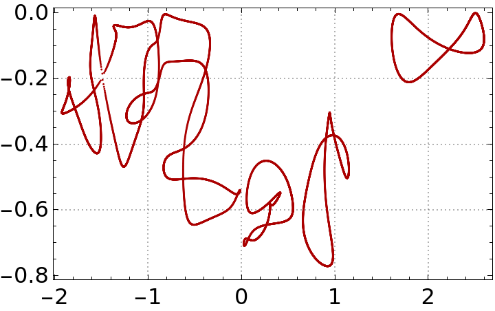
(*Plottheperiodic-boundaryspecrtuminthecomplex-energyplanefortheHamiltonianinthescatteringregionsI.*)PlotSpecI=Show[ListPlot[{#[[2]],#[[3]]}&/@Flatten[SpecIReIm,1],PlotMarkers->Markers[Darker@Red,0.013],FrameOpts[16],PlotTheme->"Detailed"]];Show[PlotSpecI,PlotRange->All]
Out[]=
Generating total Hamiltonian in scatter region I (NHSE region)and region II (Gapped scatter region) [as illustrated in Figure S6(a)]
Generating total Hamiltonian in scatter region I (NHSE region)and region II (Gapped scatter region) [as illustrated in Figure S6(a)]
Next, we construct the total Hamiltonian of the chiral chain, which comprises two distinct regions: the coexisting region (represented by the blue helix in Figure a) and the insulating region (represented by the yellow helix in Figure a). An impurity potential is introduced at the interface between these two regions. The Hamiltonian of the insulating region can be generated in the following.
μ2Scat=5.5;mz=8.5;{tsII,tpII,tsocII}={1/2,-1/2,0};HAtomII=tsocII*(KroneckerProduct[Lx,σx]+KroneckerProduct[Ly,σy]+KroneckerProduct[Lz,σz])+DiagonalMatrix[{0,0,0,0,mz,mz}]-μ2Scat*IdentityMatrix[6];H21AtomII=KroneckerProduct[tsII*Pr21+tpII*(IdentityMatrix[3]-Pr21),σ0];H32AtomII=KroneckerProduct[tsII*Pr32+tpII*(IdentityMatrix[3]-Pr32),σ0];H43AtomII=KroneckerProduct[(tsII*Pr43+tpII*(IdentityMatrix[3]-Pr43)),σ0];
Here, HIOBC and HIIOBC represent the Hamiltonians in coexisting region and insulating region, respectively, as illustrated in Fig S6 (a).
{AtomNI,AtomNII}={3*4,3*1+1}UC=6;NZI=AtomNI*UC;NZII=AtomNII*UC;HIOBC=Normal[SparseArray[{Band[{1,1},{NZI,NZI}]->{HAtomI}},{NZI,NZI}]+SparseArray[{Band[{1,1+UC},{NZI,NZI}]->{ConjugateTranspose[H21AtomI],ConjugateTranspose[H32AtomI],ConjugateTranspose[H43AtomI]}},{NZI,NZI}]+SparseArray[{Band[{1+UC,1},{NZI,NZI}]->{H21AtomI,H32AtomI,H43AtomI}},{NZI,NZI}]];HIIOBC=Normal[SparseArray[{Band[{1,1},{NZII,NZII}]->{HAtomII}},{NZII,NZII}]+SparseArray[{Band[{1,1+UC},{NZII,NZII}]->{ConjugateTranspose[H21AtomII],ConjugateTranspose[H32AtomII],ConjugateTranspose[H43AtomII]}},{NZII,NZII}]+SparseArray[{Band[{1+UC,1},{NZII,NZII}]->{H21AtomII,H32AtomII,H43AtomII}},{NZII,NZII}]];{PlotMat[HIOBC,{AtomNI-1,AtomNI-1}],PlotMat[HIIOBC,{AtomNII-1,AtomNII-1}]};
Out[]=
{12,4}
Here, we define the the impurity Hamiltonian, `HamImp’, at the interface between these two regions.
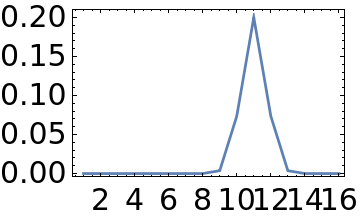
σc=1;Gauss=With{Imp=0.2},TableImp*Exp-,{x,1,AtomNI+AtomNII};HamImp=DiagonalMatrix[Flatten[KroneckerProduct[Gauss,ConstantArray[1,6]]]];Dimensions[HamImp]ListLinePlot[PaList[Diagonal[HamImp],Total[#]/UC&,UC],PlotStyle->{Thickness[0.01]},PlotRange->All,FrameOpts[15],ImageSize->Small]
2
(x-(AtomNI-1))
2
σc
Out[]=
{96,96}
Out[]=
HamScat is the total Hamiltonian composed of region I, II, and the impurity potential between them.
ScatLink=KroneckerProduct[(tsII*Pr43+tpII*(IdentityMatrix[3]-Pr43)),σ0];HamScat=ArrayFlatten[{{HIOBC,PadRight[ScatLink,{-NZI,NZII}]},{PadRight[ScatLink,{NZII,-NZI}],HIIOBC}}]+HamImp;HamScat//DimensionsPlotMat[HamScat,AtomNI+AtomNII-1];
Out[]=
{96,96}
Outcome
Outcome
Transmission Spectrum for the Chiral Chain sandwiched by right (magnetic) leads and left (normal) leads: M = +1, Rightward Current
Transmission Spectrum for the Chiral Chain sandwiched by right (magnetic) leads and left (normal) leads: M = +1, Rightward Current
In this section, we calculate the transmission coefficients at zero bias using the non-equilibrium Green’s function (NEGF) formalism. We assume that current flow induces orbital dissipation, which subsequently alters the occupation of defect states under reversed magnetism. At zero bias, orbital dissipation diminishes to zero; however, the charge trapping effect under reversed magnetism remains significant. Consequently, we effectively modify the charge trapping potential under reversed magnetism (or chirality). This modification substantially impacts the transmission coefficients, confirming the violation of Onsager’s reciprocal relation at zero bias.
Scatter region I:
Scatter region I:
We generate the Hamiltonian for region I, as illustrated by the blue chain region in Figure (a). Note that, at zero bias, the dissipation terms approach zero.
Gapped scatter region II
Gapped scatter region II
We construct the Hamiltonian for region II, which represents the insulating chiral chain.
The total Hamiltonian in scatter region I, II, and the impurity at their interface
The total Hamiltonian in scatter region I, II, and the impurity at their interface
The total Hamiltonian `HamScat’ can be constructed.
The Transmission Spectrum with left and right leads:
The Transmission Spectrum with left and right leads:
So far, we have constructed the chiral chain Hamiltonian for the scatterer region. Next, the transmission spectrum with a left ferromagnetic lead and a right normal lead can be calculated using the NEGF formalism. To proceed, we first define the surface Green’s function.
We obtain the atom Hamiltonians for the left and right leads (HSurfL and HSurfR), along with the coupling terms between the leads and the scatterer region Hamiltonian (LinkSL and LinkRS).
Here, we calculate the surface Green’s function over a frequency range from -2.5 to 4.
Calculating the retarded and advanced Green’s functions for the scatterer region Hamiltonian.
Finally, we calculate the non-equilibrium Green’s function over a range of frequencies.
Plot FigS6 e and f [or Fig2 (e) and (f) in the main text]
Plot FigS6 e and f [or Fig2 (e) and (f) in the main text]
CITE THIS NOTEBOOK
CITE THIS NOTEBOOK
Magnetochiral charge pumping due to charge trapping & skin effects in CISS
by Kai Zhang
Wolfram Community, STAFF PICKS, November 25, 2024
https://community.wolfram.com/groups/-/m/t/3327833
by Kai Zhang
Wolfram Community, STAFF PICKS, November 25, 2024
https://community.wolfram.com/groups/-/m/t/3327833